Natural transformation
Natural transformation is the most important part of the category theory. It provides a possibility to compare Functors via a standard tool.
Definitions
The natural transformation is not an easy concept compared to other ones and requires some additional preparations before we can give the formal definition.
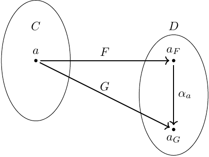
Consider 2 categories \(\mathbf{C}, \mathbf{D}\) and 2 Functors \(F: \mathbf{C} \Rightarrow \mathbf{D}\) and \(G: \mathbf{C} \Rightarrow \mathbf{D}\). If we have an Object \(a \in \mathrm{ob}(\mathbf{C})\) then it will be translated by different functors into different objects of category \(\mathbf{D}\): \(a_F = F(a), a_G = G(a) \in \mathrm{ob}(\mathbf{D})\) (see Definitions). There are 2 possible options:
There is not any Morphism that connects \(a_F\) and \(a_G\).
\(\exists \alpha_a \in \mathrm{hom}\left(a_F, a_G\right) \subset \mathrm{hom}(\mathbf{D})\).
We can of course create an artificial morphism that connects the objects but if we use natural morphisms 1 then we can get a special characteristic of the considered functors and categories. For instance if we have such morphisms then we can say that the considered functors are related to each other. As an opposite example, if there are no such morphisms then the functors can be considered as unrelated each other.
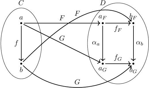
The functor is not just the object mapping but also the morphisms mapping. If we have 2 objects \(a\) and \(b\) in the category \(\mathbf{C}\) then we potentially can have a morphism \(f \in \mathrm{hom}_{\mathbf{C}}\left(a, b\right)\). In this case the morphism is mapped by the functors \(F\) and \(G\) into 2 morphisms \(f_F\) and \(f_G\) in the category \(\mathbf{D}\). As result we have 4 morphisms: \(\alpha_a, \alpha_b, f_F, f_G \in \mathrm{hom}(\mathbf{D})\). It is natural to impose additional conditions on the morphisms especially that they form a Commutative diagram (see Natural transformation): \[f_G \circ \alpha_a = \alpha_b \circ f_F.\]
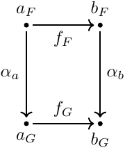
Let \(F\) and \(G\) be 2 Functors from category \(\mathbf{C}\) to the category \(\mathbf{D}\). A natural transformation from \(F\) to \(G\) is a family of Morphisms \[\alpha = \left\{ \alpha_a: F(a) \to G(a) \mid a \in \mathrm{ob}(\mathbf{C}) \right\}\] in category \(\mathbf{D}\) that satisfies the following conditions:
For every Object \(a \in \mathrm{ob}(\mathbf{C})\) the family has exactly one component \(\alpha_a \in \mathrm{hom}_{\mathbf{D}}\left(F(a), G(a)\right)\). The morphism \(\alpha_a\) is called the component of the natural transformation.
For every morphism \(f \in \mathrm{hom}(\mathbf{C})\) that connects 2 objects \(a\) and \(b\), i.e. \(f \in \mathrm{hom}_{\mathbf{C}}\left(a, b\right)\), the corresponding components \(\alpha_a\) and \(\alpha_b\) should satisfy the following condition \[f_G \circ \alpha_a = \alpha_b \circ f_F,\] where \(f_F = F(f), f_G = G(f)\). In other words the morphisms form a Commutative diagram shown on the Natural transformation.
We use the following notation (arrow with a dot) for the natural transformation between functors \(F\) and \(G\): \(\alpha: F \xrightarrow{.} G\).
The Natural transformation \(\alpha: F \xrightarrow{.} G\) is called natural isomorphism if all morphisms \(\alpha \subset \mathrm{hom}(\mathbf{D})\) are Isomorphisms in \(\mathbf{D}\)
Category of functors
The functors can be considered as objects in a special category \(\mathbf{Fun}\). The morphisms in the category are Natural transformations.
To define a category we need to define composition operation that satisfied Composition, identity morphism and verify Associativity.
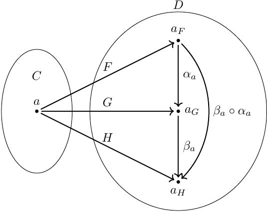
For the composition consider 2 Natural transformations \(\alpha, \beta\) and consider how they act on an object \(a \in \mathrm{ob}(\mathbf{C})\) (see Category of functors). We always can construct the composition \(\beta_a \circ \alpha_a\) i.e. we can define the composition of natural transformations \(\alpha, \beta\) as \(\beta \circ \alpha = \left\{ \beta_a \circ \alpha_a | a \in \mathrm{ob}(\mathbf{C}) \right\}\).
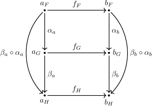
The natural transformation is not just object mapping but also morphism mapping. We shall require that all morphisms shown on Category of functors commute. The composition defined in such way is called Vertical composition.
Let \(F,G,H\) are functors between categories \(\mathbf{C}\) and \(\mathbf{D}\). Also we have \(\alpha : F \xrightarrow{.} G, \beta: G \xrightarrow{.} H\) - natural transformations. We can compose the \(\alpha\) and \(\beta\) as follows \[\beta \circ \alpha: F \xrightarrow{.} H.\] This composition is called vertical composition.
Let \(\mathbf{C}\) and \(\mathbf{D}\) are 2 categories. The category that contains functors \(F: \mathbf{C} \Rightarrow \mathbf{D}\) as objects and Natural transformation as morphisms is called as functor category. The morphism composition is the Vertical composition in the category. The functor category between categories \(\mathbf{C}\) and \(\mathbf{D}\) is denoted as \([\mathbf{C}, \mathbf{D}]\).
Uniqueness of Natural transformation is the same to uniqueness of morphisms in the target category as soon as the natural transformation is a set of Morphisms in it. This fact leads to the following examples for initial and terminal objects in Fun category.
Let \([\mathbf{C}, \mathbf{D}]\) is the functor category between \(\mathbf{C}\) and \(\mathbf{D}\). If \(t \in \mathrm{ob}(\mathbf{D})\) is the Terminal object in the category \(\mathbf{D}\) then the Constant functor \(\Delta_t\) is the Terminal object in the category \([\mathbf{C}, \mathbf{D}]\) ((https://math.stackexchange.com/users/455216/enkidu), n.d.).
Let \([\mathbf{C}, \mathbf{D}]\) is the functor category between \(\mathbf{C}\) and \(\mathbf{D}\). If \(i \in \mathrm{ob}(\mathbf{D})\) is the Initial object in the category \(\mathbf{D}\) then the Constant functor \(\Delta_i\) is the Initial object in the category \([\mathbf{C}, \mathbf{D}]\) ((https://math.stackexchange.com/users/455216/enkidu), n.d.).
Operations with natural transformations
Vertical composition is not the unique way to compose 2 Natural transformations. Another option is also possible.
If we have 2 pairs of functors. The first one \(F,G: \mathbf{C} \to \mathbf{D}\) and another one \(J,K: \mathbf{D} \Rightarrow \mathbf{E}\). We also have a natural transformation between each pair: \(\alpha : F \xrightarrow{.} G\) for the first one and \(\beta : J \xrightarrow{.} K\) for the second one. We can create a new transformation \[\alpha \star \beta: J \circ F \xrightarrow{.} K \circ G\] that is called horizontal composition. For every object \(a \in \mathrm{ob}(\mathbf{C})\) its component is defined as follows: \[(\alpha \star \beta)_a = \beta_{G(a)} \circ J(\alpha_a) = K(\alpha_a) \circ \beta_{F(a)}.\] The equality of the 2 expressions follows from naturality of \(\beta\). Note that we use a special symbol \(\star\) for the composition.
If we have the same pair of functors as in Horizontal composition then we can consider the functors as Objects of 3 categories: \(\mathbf{\mathcal{A}} = \left[\mathbf{C}, \mathbf{D}\right], \mathbf{\mathcal{B}} = \left[\mathbf{D}, \mathbf{E}\right]\) and \(\mathbf{\mathcal{C}} = \left[\mathbf{C}, \mathbf{E}\right]\)
We can construct a Bifunctor \(\otimes: \mathbf{\mathcal{A}} \times \mathbf{\mathcal{B}} \Rightarrow \mathbf{\mathcal{C}}\) where for each pair of objects \(F \in \mathrm{ob}(\mathbf{\mathcal{A}}), J \in \mathrm{ob}(\mathbf{\mathcal{B}})\) we get another object from \(\mathbf{\mathcal{C}}\). We used the ordinary functor’s composition as the operation for objects mapping. I.e. \[\otimes: F \times J \to J \circ F \in \mathrm{ob}(\mathbf{\mathcal{C}}).\]
The bifunctor is not just a map for objects. There is also a map between morphisms. Thus if we have 2 Morphisms: \(\alpha : F \to G\) and \(\beta : J \to K\) then we can construct the following mapping \[\otimes: \alpha \times \beta \to \alpha \star \beta \in \mathrm{hom}(\mathbf{\mathcal{C}}).\]
As result we just introduced mapping \(\otimes\) as a Bifunctor in the category of functors.
If we have 3 categories \(\mathbf{B}, \mathbf{C}, \mathbf{D}\), Functors \(F,G: \mathbf{C} \Rightarrow \mathbf{D}\), \(H: \mathbf{B} \to \mathbf{C}\) and Natural transformation \(\alpha: F \xrightarrow{.} G\) then we can construct a new natural transformations: \[\alpha H : F \circ H \xrightarrow{.} G \circ H\] that is called left whiskering of functor and natural transformation (authors 2018).
If we have 3 categories \(\mathbf{C}, \mathbf{D}, \mathbf{E}\), Functors \(F,G: \mathbf{C} \Rightarrow \mathbf{D}\), \(H: \mathbf{D} \to \mathbf{E}\) and Natural transformation \(\alpha: F \xrightarrow{.} G\) then we can construct a new natural transformations: \[H \alpha : H \circ F \xrightarrow{.} H \circ G\] that is called right whiskering of functor and natural transformation (authors 2018).
If \(F: \mathbf{C} \Rightarrow \mathbf{D}\) is a Functor then we can define identity natural transformation \(\mathbf{1}_{F \xrightarrow{.} F}\) that maps any Object \(a \in \mathrm{ob}(\mathbf{C})\) into Identity morphism \(\mathbf{1}_{F(a) \to F(a)} \in \mathrm{hom}(\mathbf{D})\).
With Identity natural transformation we can redefine Left whiskering and Right whiskering via Horizontal composition as follows.
For left whiskering: \[\alpha H = \mathbf{1}_{H \xrightarrow{.} H} \star \alpha\]
For right whiskering: \[H \alpha = \alpha \star \mathbf{1}_{H \xrightarrow{.} H}\]
Polymorphism and natural transformation
Polymorphism plays a certain role in programming languages. Category theory provides several facts about polymorphic functions which are very important.
Polymorphism is parametric if all function instances behave uniformly i.e. have the same realization. The functions which satisfy the parametric polymorphism requirements are parametrically polymorphic.
Polymorphism is ad-hoc if the function instances can behave differently dependently on the type they are being instantiated with.
Let \(\mathbf{T}\) be a category of types and total functions. Let \(F,G: \mathbf{T} \Rightarrow \mathbf{T}\) be covariant type constructors whose relational interpretations map the graph relation of every function \(f: a \to b\) to the graph relations of \(F(f)\) and \(G(f)\). A Parametrically polymorphic function \[p: \forall a.\;F(a) \to G(a)\] defines a Natural transformation \(p: F \xrightarrow{.} G\).
Proof. For every type \(a\) the function instance \(p_a: F(a) \to G(a)\) is a Morphism in \(\mathbf{T}\). Therefore we already have the components that are required by Natural transformation.
It remains to verify the naturality condition. Let \(f: a \to b\) be a morphism in \(\mathbf{T}\). Reynolds’ abstraction theorem (Reynolds 1983) states that a parametrically polymorphic function preserves relations between type instances. We apply this statement to the graph relation of \(f\): \[x \mathrel{R_f} y \iff f(x) = y.\] By the assumption on \(F\) and \(G\), this graph relation is mapped to the graph relations of \(F(f)\) and \(G(f)\). Thus, if \(x \in F(a)\), then \(x\) and \(F(f)(x)\) are related by the relation obtained from \(R_f\) by the type constructor \(F\). Parametricity of \(p\) implies that \(p_a(x)\) and \(p_b(F(f)(x))\) are related by the relation obtained from \(R_f\) by the type constructor \(G\). But this relation is the graph relation of \(G(f)\). Thus \[G(f)(p_a(x)) = p_b(F(f)(x)).\] Since this equality holds for every \(x \in F(a)\), we get \[G(f) \circ p_a = p_b \circ F(f).\] This is exactly the naturality condition from (Natural transformation). Therefore the family of components \(p = \{p_a\}_{a \in \mathrm{ob}(\mathbf{T})}\) is a Natural transformation. ◻
\(\mathbf{Hask}\) category
Many pure polymorphic functions in Haskell are Parametrically polymorphic functions 2.
Consider the following function
safeHead :: [a] -> Maybe a
safeHead [] = Nothing
safeHead (x:xs) = Just x
The function is parametrically polymorphic and by Reynolds is Natural transformation (see Parametrically polymorphic function).
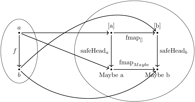
Therefore from the definition of the natural transformation (Natural transformation) we have
fmap f . safeHead = safeHead . fmap fI.e. applying safeHead first and then mapping inside the Maybe gives the same result as mapping over the list first and then applying safeHead.
The statement can be verified directly. For empty list we have
(fmap f . safeHead) []
-- equivalent to
fmap f Nothing
-- equivalent to
Nothing
On the other side
(safeHead . fmap f) []
-- equivalent to
safeHead []
-- equivalent to
Nothing
For a non-empty list we have
(fmap f . safeHead) (x:xs)
-- equivalent to
fmap f (Just x)
-- equivalent to
Just (f x)
On the other side
(safeHead . fmap f) (x:xs)
-- equivalent to
safeHead (f x : fmap f xs)
-- equivalent to
Just (f x)
Using the fact that fmap f is an expensive operation if it is applied to the whole list, we can conclude that the first approach is more productive in a strict setting: it applies fmap f only to the Maybe result. Such transformation allows compiler to optimize the code. 3
Discussion
Register with a username and password to join the discussion.