Curry-Howard-Lambek correspondence
There is an interesting correspondence between computer programs and mathematical proofs. Different types of logic correspond to different computational models. This allows to build a theory of computation on the base of math logic. First of all consider a category of proofs
\(\mathbf{Proof}\) category
Proposition is a statement that either true or false.
There are 2 main propositions
A true statement is one that is correct, either in all cases or at least in the sample case (Quist, n.d.).
and
A false statement is one that is not correct (Quist, n.d.).
There is an example of correct (true) proposition \[\forall n \in \mathbb{R}: n^2 \ge 0\]
There is an example of incorrect (false) proposition \[\exists n \in \mathbb{R}: n^2 < 0.\]
The expression \(\forall n \in \mathbb{C}: n^2 \ge 0\) is not a good example of a false proposition in standard math because \(\mathbb{C}\) has no standard order for the comparison \(\ge\).
An implication is a Proposition of the form \(P \implies Q\) i.e. if \(P\) then \(Q\) (Leighton and Rubinfeld, n.d.).
The main logical deduction rule is the following
If \(P\) is true and \(P \implies Q\) is true then \(Q\) is also true. The rule is often written as (Leighton and Rubinfeld, n.d.) \[\frac{ \begin{array}{c} P \\ P \implies Q \end{array} }{Q}\] where if statements above the line are true then the statement below the line is also true.
Proof is a verification (Leighton and Rubinfeld, n.d.) of a Proposition by a chain of logical deduction from a base set of axioms.
Propositions can be combined into new propositions via the following logical operations
Conjunction or logical AND is the operation with following rules
| \(a\) | \(b\) | \(a \land b\) |
|---|---|---|
| True | True | True |
| True | False | False |
| False | True | False |
| False | False | False |
Disjunction or logical OR is the operation with following rules
| \(a\) | \(b\) | \(a \lor b\) |
|---|---|---|
| True | True | True |
| True | False | True |
| False | True | True |
| False | False | False |
Operations in Boolean logic follow the distributive law: \[a \land ( b \lor c) = (a \land b) \lor (a \land c)\] i.e. the operation \(\land\) corresponds to multiplication and \(\lor\) to sum. Therefore the \(\mathbf{Proof}\) can be considered as a Distributive category.
The \(\mathbf{Proof}\) category is a category where Propositions are Objects and Proofs are Morphisms. I.e. proofs are used as connectors between different propositions.
Consider different objects and constructions of the proof (logic) theory from the categorical point of view
The false statement can be considered as the initial object because for any other statement there is a proof from the false statement to that one. If we identify proofs with the same entailment or work in a proof-irrelevant setting, this proof is unique.
The true statement can be considered as the terminal object
Conjunction can be considered as Product in Proof category.
Disjunction can be considered as Sum in Proof category.
Thus we can declare the following correspondence (see Proof) between logic proofs and Cartesian closed category and therefore also between programming languages.
width=1
| Proof category | Programming language | Cartesian closed category |
|---|---|---|
| Proposition | Type | Object |
| Proof | Program or term | Morphism |
| Implication | Function type | Exponential |
| Conjunction | Product type | Product |
| Disjunction | Sum type | Sum |
| True | unit type | Terminal object |
| False | bottom type | Initial object |
Linear logic and Linear types
Linear logic (Di Cosmo and Miller 2016) is a refinement of classical logic where the usage of a statement becomes important. In classical logic we can use the same statement several times or ignore it. In linear logic a statement can be considered as a resource. If a resource is used in an Implication, then it cannot be used again without an explicit rule that permits copying.
This point of view is useful for computations where values represent real resources. For example, a file handle, a lock, or a communication channel should not be silently duplicated or forgotten. Linear types add the same discipline to a programming language: a value of a linear type has to be used exactly once. Thus the type checker can verify resource usage statically, which is especially useful in concurrent programs.
Quantum logic and quantum computation
Different modifications of logic rules give us new computational models. One of example is the quantum computations. The quantum logic differs from Boolean one in the missing distributive law (Proof).
We can use the Heisenberg inequality to illustrate the violation of the law. Consider a particle with 2 possible positions range and 1 possible momentum range. The event \(P\) is that momentum has range \(\Delta p\). The event \(Q_{1,2}\) is that position is in the corresponding range \(\Delta q_{1,2}\) (see Quantum logic and quantum computation).
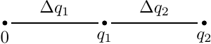
Heisenberg inequality says \[\Delta p \Delta q_{1,2} \geq \frac{\hbar}{2}\] i.e. the following 2 events \(P\land Q_{1,2}\) are forbidden as soon as (see Quantum logic and quantum computation): \[\Delta p \Delta q_1 = \frac{\hbar}{3}\] and \[\Delta p \Delta q_2 = \frac{\hbar}{3}\] i.e. \[P \land Q_1 = P \land Q_2 = \mbox{False}\] from other side the event \(P \land (Q_1 \lor Q_2)\) can be \(\mbox{True}\) as soon as (see Quantum logic and quantum computation) \[\Delta p (\Delta q_1 + \Delta q_2) = \frac{2\hbar}{3} > \frac{\hbar}{2}.\] Therefore we have distributive law (Proof) violation \[P \land (Q_1 \lor Q_2) \ne (P \land Q_1 ) \lor (P \land Q_2).\]
Discussion
Register with a username and password to join the discussion.