Base definitions
Definitions
The chapter provides you with base definitions that will be widely used in the book later. We will give definitions for Object, Morphism, Category and also provide you with several important examples, such as the Set category.
Object
A class is a collection of sets (or sometimes other mathematical objects) that can be unambiguously defined by a property that all its members share.
Every set determines a class, but not every class is a set. For example, the class of all sets is a proper class. Treating it as a set would lead to contradictions such as Russell’s paradox.
In ZFC, a class is notation for all sets that satisfy a given property; it is not a separate mathematical object. Therefore a proper class cannot be an element of a set or of another class. Groups and vector spaces can be represented by sets. Small categories can also be represented by sets, whereas large categories, such as \(\mathbf{Set}\), are described by proper classes.
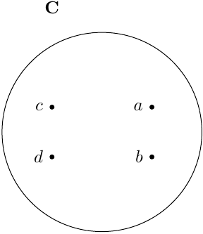
In category theory an object is considered as something that does not have internal structure (aka point) but has a property that makes different objects belong to the same Class.
Morphism
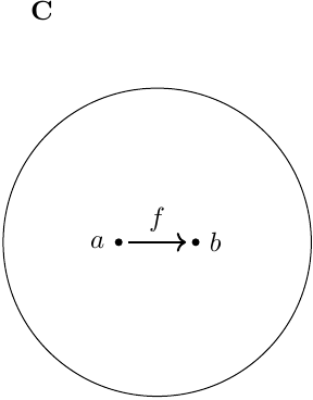
Morphism is a kind of relation between 2 Objects.
A relation between two Objects \(a\) and \(b\) \[f: a \rightarrow b\] is called a morphism. A morphism assumes a direction i.e. one Object (\(a\)) is called the source or Domain and another one (\(b\)) the target or Codomain.
The Set of all morphisms between objects \(a\) and \(b\) is denoted as \(\mathrm{hom}\left(a, b\right)\).
The important remark about morphisms is below.
A morphism has to be considered as a separate piece of structure, not only as a pair of source and target objects. We will avoid writing a general morphism in the set-theoretic form \(f(a) = b\), because this notation treats the objects \(a\) and \(b\) as elements and hides the possibility of different parallel morphisms. Let \(f_1: a \to b\) and \(f_2: a \to b\) be two different morphisms; they have the same source and target, but this does not imply \(f_1 = f_2\).
For instance, in \(\mathbf{Set}\) the functions \(f_1, f_2: \mathbb{R} \to \mathbb{R}\) defined by \(f_1(x) = x\) and \(f_2(x) = -x\) have the same domain and codomain, but they are different Morphisms.
Given a Morphism \(f: a \to b\), the Object \(a\) is called domain and denoted as \(\operatorname{dom}f\).
Given a Morphism \(f: a \to b\), the Object \(b\) is called codomain and denoted as \(\operatorname{cod}f\).
Morphisms have several properties. 1
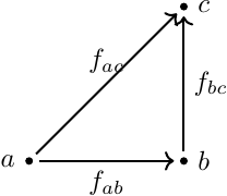
If there are 3 Objects \(a, b, c\) and 2 Morphisms \[\begin{aligned} f_{ab} : a \rightarrow b, \nonumber \\ f_{bc} : b \rightarrow c \nonumber \end{aligned}\] then there exists a Morphism (see Morphism) \[f_{ac} : a \rightarrow c\] such that \[f_{ac} = f_{bc} \circ f_{ab}\]
The equation \[f_{ac} = f_{bc} \circ f_{ab}\] means that we apply \(f_{ab}\) first and then we apply \(f_{bc}\) to the result of the application i.e. if our objects are sets and \(x \in a\) then \[f_{ac} ( x ) = f_{bc} ( f_{ab} ( x ) ),\] where \(f_{ab} ( x ) \in b, f_{ac} ( x ) \in c\).
The Morphism Composition should follow associativity property: \[f_{ce} \circ (f_{bc} \circ f_{ab}) = (f_{ce} \circ f_{bc}) \circ f_{ab} = f_{ce} \circ f_{bc} \circ f_{ab}.\]
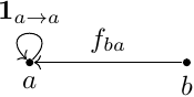
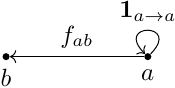
For every Object \(a\) there is a special Morphism \(\mathbf{1}_{a \to a} : a \rightarrow a\) with the following properties: \(\forall f_{ba} : b \rightarrow a\) (see Morphism) \[\mathbf{1}_{a \to a} \circ f_{ba} = f_{ba}\] and \(\forall f_{ab} : a \rightarrow b\) (see Morphism) \[f_{ab} \circ \mathbf{1}_{a \to a} = f_{ab}.\] This morphism is referred to as identity morphism.
Note that Identity morphism is unique, see Identity is unique below.
A diagram in a category \(\mathbf{C}\) is a collection of vertices and directed edges where the vertices correspond to the objects of \(\mathbf{C}\) and edges consistently correspond to the morphisms (see Diagram).
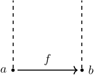
Consistently means that for an edge named as \(f\) has endpoints labeled \(a\) and \(b\), where \(f\) is a morphism of \(\mathbf{C}\), \(a\) is Domain of \(f\) and \(b\) is Codomain of \(f\).
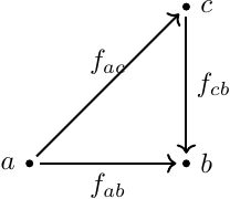
A Diagram of category \(\mathbf{C}\) is said to commute if all directed paths in the diagram with the same start and endpoint lead to the same result by composition.
The trivial example of Commutative diagram is Composition for \(f_{ab} = f_{cb} \circ f_{ac}\):
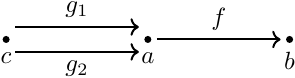
If \(\forall g_1, g_2\) the equation \[f \circ g_1 = f \circ g_2\] leads to \[g_1 = g_2\] then \(f\) is called monomorphism (see Monomorphism). The monomorphism between \(a\) and \(b\) is denoted as \(f: a \hookrightarrow b\) (see also Injection or “one-to-one” functions).
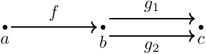
If \(\forall g_1, g_2\) the equation (see Epimorphism) \[g_1 \circ f = g_2 \circ f\] leads to \[g_1 = g_2\] then \(f\) is called epimorphism (see also Surjection or “onto” functions).
A Morphism \(f: a \to b\) is called isomorphism if \(\exists g: b \to a\) such that \(f \circ g = \mathbf{1}_{b \to b}\) and \(g \circ f = \mathbf{1}_{a \to a}\). If there is an isomorphism \(f\) between objects \(a\) and \(b\) then it is denoted by \(a \cong_f b\).
There can be many different Isomorphisms between 2 Objects.
If there is a unique isomorphism between 2 objects \(a\) and \(b\) then the objects can be treated as the same object for categorical purposes, although they are not necessarily equal as objects.
Category
A category \(\mathbf{C}\) consists of
Class of Morphisms \(\mathrm{hom}(\mathbf{C})\) defined for \(\mathrm{ob}(\mathbf{C})\), i.e. each morphism \(f_{ab}\) from \(\mathrm{hom}(\mathbf{C})\) has both source \(a\) and target \(b\) from \(\mathrm{ob}(\mathbf{C})\)
For any Object \(a\) there should be unique Identity morphism \(\mathbf{1}_{a \to a}\). Any morphism should satisfy Composition and Associativity axioms (see example in Category).
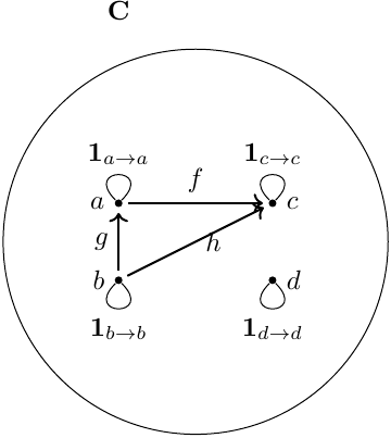
The set of morphisms between objects \(a\) and \(b\) in the category \(\mathbf{C}\) will be denoted as \(\mathrm{hom}_{\mathbf{C}}\left(a, b\right)\). The set will be denoted as \(\mathrm{hom}\left(a, b\right)\) if the exact category does not matter.
The Category can be considered as a way to represent a structured data. Objects are the data and Morphisms form the structure that connects the data.
If \(\mathbf{C}\) is a Category then opposite (or dual) category \(\mathbf{C}^{op}\) is constructed in the following way: Objects are the same, but the Morphisms are inverted i.e. if \(f \in \mathrm{hom}(\mathbf{C})\) and \(\operatorname{dom}f = a, \operatorname{cod}f = b\) (see Domain, Codomain), then the corresponding morphism \(f^{op} \in \mathrm{hom}(\mathbf{C^{op}})\) has \(\operatorname{dom}f^{op} = b, \operatorname{cod}f^{op} = a\) (see Category)
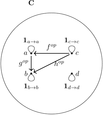
Composition on \(C^{op}\)
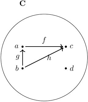
As you can see from Category the Composition is reverted for Opposite category. If \(f,g,h = f \circ g \in \mathrm{hom}(\mathbf{C})\) then \(f \circ g\) translated into \(g^{op} \circ f^{op}\) in opposite category.
A category \(\mathbf{C}\) is called small if both \(\mathrm{ob}(\mathbf{C})\) and \(\mathrm{hom}(\mathbf{C})\) are Sets
A category \(\mathbf{C}\) is called locally small if for every 2 Objects \(a,b \in \mathrm{ob}(\mathbf{C})\) the collection \(\mathrm{hom}_{\mathbf{C}}\left(a, b\right)\) of all Morphisms from \(a\) to \(b\) is a Set. The set is called Homset.
The homset \(\mathrm{hom}_{\mathbf{C}}\left(a, b\right)\) is the Set of Morphisms from \(a\) to \(b\) in a Locally small category.
A category \(\mathbf{C}\) is called large if it is not a Small category. An example of a large category is Set category
The category that does not contain any Objects and as result does not contain any Morphisms is called Empty category ((https://math.stackexchange.com/users/301130/user84563), n.d.).
The category that contains only one Object and only one Morphism (Identity morphism) is called Trivial category.
There are several examples of categories below that will also be actively used later in the book:
\(\mathbf{Set}\) category example: see Set
Programming languages (Haskell, C
++, Scala) examples: see Programming languages examplesQuantum mechanics example: see Quantum mechanics examples
\(\mathbf{Set}\) category example
The category of sets is the most important example because it connects our usual knowledge about sets with the category theory.
Set is a collection of distinct objects. The objects are called the elements of the set.
The set will be denoted by a capital letter in the book, for instance \(A\). The elements of a set will be denoted by small letters: \(a \in A\).
The definition of Set was given above is incomplete. There are several additional axioms should be applied for the complete definition. Different sets of axioms can be used. In our case we consider so called Zermelo—Fraenkel set theory with the axiom of Choice or ZFC (Wikipedia contributors 2018b). The system of axioms allows us to avoid different logical paradoxes of the set theory, for instance well known Russell’s paradox (Wikipedia contributors 2018a).
The number of elements in the Set \(A\) is called cardinality and is denoted as \(\left|A\right|\).
If \(A\) and \(B\) are two sets then we can define a new set \(A \times B = \left\{(a,b)|a \in A, b \in B\right\}\) that is called as the cartesian product.
If \(A\) and \(B\) are 2 Sets then a subset of the Cartesian product \(A \times B\) is called as binary relation \(R\) between the 2 sets, i.e. \(R \subset A \times B\).
Example of binary relation is shown on Binary relation. There is a relation \(R\) between 2 sets \(A\) and \(B\). The relation maps \(a_1\) into two different values \(b_1\) and \(b_2\).
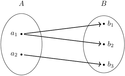
Function \(f\) is a special type of Binary relation. I.e. if \(A\) and \(B\) are 2 Sets then a subset of \(A \times B\) is called function \(f\) between the 2 sets if \(\forall a \in A \, \exists! b \in B\) such that \((a,b) \in f\).
The main difference between Function and Binary relation is that Binary relation allows mapping an argument into more than one value (see Binary relation). From other side Function definition does not allow such “multi value”.
In the Set category we consider a Class of Sets where Objects are the Sets and Morphisms are Functions between the sets. The Identity morphism is the trivial function such that \(\forall x \in X: \mathbf{1}_{X \to X}(x) = x\). Composition is the functions composition (see Set)
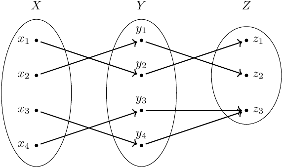
In general case when we say \(\mathbf{Set}\) category we assume the class of all sets. The class of all sets is not a set itself because famous Russell’s paradox (Wikipedia contributors 2018a) can be applied. To avoid such situations we consider a limitation that is applied on our construction as it was mentioned at Set, especially ZFC (Wikipedia contributors 2018b) is applied. If we take into consideration the limitation then the \(\mathbf{Set}\) category is a Large category.
The singleton is a Set with only one element.
Given a function \(f: X \to Y\), the set \(X\) is the domain. I.e. \(\operatorname{dom} f = X\)
Given a function \(f: X \to Y\), the set \(Y\) is the codomain. I.e. \(\operatorname{cod}f = Y\)
The image of a function \(f: X \to Y\) is a subset of Codomain \(Y\) such that for every element in the subset there is an element in Domain \(X\) that maps into the subset: \[\operatorname{Im}{f} = \{y \in Y| y = f(x) \mbox{ for some } x \in X\}\]
The function \(f: X \rightarrow Y\) is surjective (or “onto”) if \(\forall y \in Y\), \(\exists x \in X\) such that \(f\left(x\right) = y\) (see Surjection, Set).
An example of a surjective function is shown in Surjection. Note that the function in the figure is not an Injection. You can find an example of a function that is Surjection as well as Injection (aka Bijection) in Set.
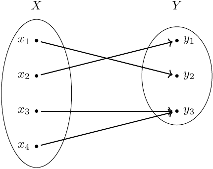
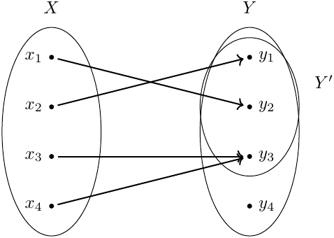
Surjection and Epimorphism are related each other. Consider a non-surjective function \(f: X \rightarrow Y\) and let \(Y' \subset Y\) be the image of \(f\) (see Surjection vs Epimorphism). One can conclude that \(f\) is not an Epimorphism. Let \(Z = \{0, 1\}\). We can define two functions \(g_1, g_2 : Y \to Z\) such that \(g_1(y) = g_2(y)\) for all \(y \in Y'\) but \(g_1 \ne g_2\) on at least one element of \(Y \setminus Y'\). As soon as \(f(x) \in Y'\) for all \(x \in X\), we always have \(g_1(f(x)) = g_2(f(x))\). I.e. \[g_1 \circ f = g_2 \circ f,\] but \(g_1 \ne g_2\). Thus every Epimorphism in \(\mathbf{Set}\) has to be a Surjection. Conversely, every Surjection is an Epimorphism in the \(\mathbf{Set}\) category. The full proof can be found at (ProofWiki 2018b).
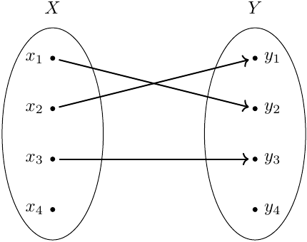
The function \(f: X \rightarrow Y\) is injective (or “one-to-one” function) if \(\forall x_1, x_2 \in X\), such that \(x_1 \ne x_2\) then \(f\left(x_1\right) \ne f\left(x_2\right)\) (see Injection, Set).
An example of an injective function is shown in Injection. Note that the function in the figure is not a Surjection. You can find an example of a function that is Surjection as well as Injection (aka Bijection) in Set.
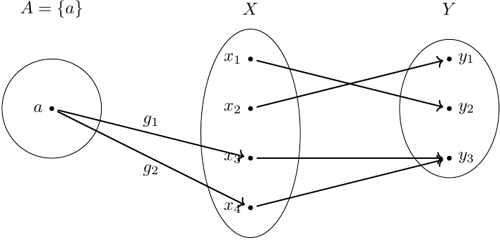
Injection and Monomorphism are related each other. Consider a non-injective function \(f: X \rightarrow Y\) (see Set). One can conclude that it is not a Monomorphism because there are \(x_1, x_2 \in X\) such that \(x_1 \ne x_2\) but \(f(x_1) = f(x_2)\). Let \(A = \{a\}\). We can define two functions \(g_1, g_2: A \to X\) such that \(g_1(a) = x_1\) and \(g_2(a) = x_2\). Thus \(g_1 \ne g_2\) but \[f \circ g_1 = f \circ g_2.\] Thus every Monomorphism in \(\mathbf{Set}\) has to be an Injection. Conversely, every Injection is a Monomorphism in the \(\mathbf{Set}\) category. The full proof can be found at (ProofWiki 2018a).
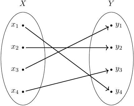
The function \(f: X \rightarrow Y\) is bijective (or “one-to-one” correspondence) if it is an Injection and a Surjection (see Set).
There is a question what is the categorical analog of a single Set. Main characteristic of a category is a structure but the Set by definition does not have a structure. Which category does not have any structure? The answer is the Discrete category.
Discrete category is a Category where Morphisms are only Identity morphisms.
Programming languages examples
Functions are the most important constructions in programming languages. They convert elements 2 of one type into elements of another one.
The function is pure if it’s execution give the same results independently from the environment.
Categorical view to programming languages assumes types as Objects and functions as Morphisms. The critical requirements for such consideration is that the functions have to be Pure functions (without side effects). This requirement mainly is satisfied by functional languages such as Haskell and Scala.
From other side the functional languages use lazy evaluation to improve their performance. The laziness can also make category theory axiom invalid (see Haskell lazy evaluation below).
Each Haskell type has a special value \(\bot\). The fact that the value and the lazy evaluations are parts of the language, make several category law invalid, for instance Identity morphism behaviour become invalid in specific cases.
The following code
seq undefined Trueproduces undefined But the following
    seq (id.undefined) True
    seq (undefined.id) True
produces True in both cases. As result we have 3
    id . undefined /= undefined
    undefined . id /= undefined,
i.e. (Identity morphism) and (Identity morphism) are not satisfied.
In the example we used the seq function that has the following signature
seq :: a -> b -> bi.e. it takes two arguments and returns the second one. It also evaluates the first argument: \[\begin{aligned} seq(\bot, b) = \bot, \nonumber \\ seq(a, b) = b. \nonumber \end{aligned}\]
Strictly speaking neither Haskell (pure functional language) nor
C++ can be considered as a category in general. For the
first approximation a functional language (Haskell, Scala) can be
considered as a category if we avoid to use functions with side effects
(mainly for Scala) and use strict, not lazy, evaluations (for both
Haskell and Scala). Lets take the fact into consideration and define
categories for 3 languages
The objects in the \(\mathbf{Hask}\) category are Haskell types and morphisms are functions. We use only strict (not lazy) evaluations for functions in the category.
The objects in the \(\mathbf{Scala}\) category are Scala types and morphisms are functions. We don’t define functions that have side effects in the category. I.e. the functions are Pure functions. We also use only strict (not lazy) evaluations for functions in the category.
The objects in the \(\mathbf{C\texttt{++}}\) category are
C++ types and morphisms are functions. We don’t define
functions that have side effects in the category. I.e. the functions are
Pure functions.
In any case we can construct a simple toy category that can be easy implemented in any language. Particularly we shall look into category with 3 Objects that are types: Int, Bool, String. There are also several Morphisms (functions) between them (see Programming languages examples).
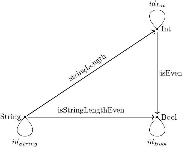
\(\mathbf{Hask}\) toy category
Types in Haskell are considered as Objects. Functions are considered as Morphisms. We are going to implement Category from Programming languages examples.
The function isEven converts Int type into Bool.
    isEven :: Int -> Bool
    isEven x = x `mod` 2 == 0
There is also Identity morphism that is defined as follows
    id :: a -> a
    id x = x
If we have an additional function
    stringLength :: String -> Int
    stringLength x = length x
then we can create a Composition
    isStringLengthEven :: String -> Bool
    isStringLengthEven = isEven . stringLength
\(\mathbf{Scala}\) toy category
we shall use the same trick as in Hask toy category and will assume types in Scala as Objects, functions as Morphisms. We also are going to implement Category from Programming languages examples.
    object Category {
      def id[A]: A => A = a => a
      def compose[A, B, C](g: B => C, f: A => B):
          A => C = g compose f

      val isEven = (i: Int) => i % 2  == 0
      val stringLength = (s: String) => s.length
      val isStringLengthEven = (s: String) =>
          compose(isEven, stringLength)(s)
    }
The usage example is below
    class CategorySpec extends Properties("Category") {
      import Category._
      import Prop.forAll

      property("composition") = forAll { (s: String) =>
        isStringLengthEven(s)  == isEven(stringLength(s))
      }

      property("right id") = forAll { (i: Int) =>
        isEven(i)  == compose(isEven, id[Int])(i)
      }

      property("left id") = forAll { (i: Int) =>
        isEven(i)  == compose(id[Boolean], isEven)(i)
      }
    }
\(\mathbf{C\texttt{++}}\) toy category
we shall use the same trick as in Hask toy
category and will assume types in C++ as Objects, functions as Morphisms. we shall implement Category from Programming languages examples.
Lets define 2 functions as follows:
    auto isEven = [](int x) {
      return x % 2 == 0;
    };

    auto stringLength = [](std::string s) {
      return static_cast<int>(s.size());
    };
Then we can define composition:
    // h = g . f
    template <typename A, typename B>
    auto compose(A g, B f) {
      auto h = [f, g](auto a) {
        auto b = f(a);
        auto c = g(b);
        return c;
      };
      return h;
    };
The Identity morphism:
auto id = [](auto x) { return x; };The usage examples are the following:
    auto isStringLengthEven = compose<>(isEven, stringLength);

    auto isStringLengthEvenL = compose<>(id, isStringLengthEven);

    auto isStringLengthEvenR = compose<>(isStringLengthEven, id);
Such construction will always provides us a category until we use pure function (functions without effects).
Quantum mechanics examples
The most critical property of quantum system is the superposition principle. The Set category cannot be used for it because it does not satisfy the principle but a simple modification of the \(\mathbf{Set}\) category does.
we shall consider a class of sets (same as Set category) i.e. Sets as Objects. Instead of Functions we shall use Binary relations as Morphisms.
The \(\mathbf{Rel}\) category is similar to the finite dimensional Hilbert space especially because it assumes some kind of superposition. Really consider \(\mathbf{Rel}\) - the \(\mathbf{Rel}\) category. \(X, Y \in \mathrm{ob}(\mathbf{Rel})\) - 2 sets which consist of different elements. Let \(f: X \to Y\) - Morphism. Each element \(x \in X\) is mapped to a subset \(Y' \subset Y\). The \(Y'\) can be Singleton (in this case no differences with Set category) but there can be a situation when \(Y'\) consists of several elements. In the case we shall get some kind of superposition that is analogous to quantum systems.
In quantum mechanics we use Hilbert spaces that are Vector spaces under Field of complex numbers \(\mathbb{C}\).
The Hilbert space is a complex Vector space with an inner product whose values are complex numbers (\(\mathbb{C}\)), complete with respect to the norm induced by this inner product.
Later we shall consider only finite dimensional Hilbert spaces. We shall denote a Hilbert space of dimension \(n\) as \(\mathcal{H}_n\). Obviously \(\mathcal{H}_1 = \mathbb{C}\).
Each Hilbert space \(\mathcal{H}\) has an associated dual space \(\mathcal{H}^\ast\) that consists of linear functionals.
Consider a ket-vector \(\ket{\psi} \in \mathcal{H}\). Then the corresponding vector from Dual space is called bra-vector \(\bra{\psi} \in \mathcal{H}^\ast\). From the definition of dual space the bra-vector is a linear functional i.e. \[\bra{\psi} : \mathcal{H} \to \mathbb{C},\] \(\forall \ket{\phi} \in \mathcal{H}\) we have \(\bra{\psi}\left(\ket{\phi}\right) = \left(\ket{\psi}, \ket{\phi}\right)\) - inner product that is often written as \(\bra{\psi}\ket{\phi}\).
The transformation between 2 Hilbert spaces that preserves the structure is called linear map or linear transformations.
The linear map between 2 Hilbert spaces \(\mathcal{A}\) and \(\mathcal{B}\) is a mapping \(f: \mathcal{A} \to \mathcal{B}\) that preserves additions \[f(a_1 + a_2) = f(a_1) + f(a_2),\] and scalar multiplications: \[f(c \cdot a) = c \cdot f(a)\] where \(a,a_1,a_2 \in \mathcal{A}\) and \(f(a), f(a_1), f(a_2) \in \mathcal{B}\).
Note that a Linear map does not necessarily preserve the inner product. Let us consider \(\mathcal{H}_1 = \mathbb{C}\) with the usual inner product and a linear map \(f: \mathbb{C} \to \mathbb{C}\) defined as \(f(z) = 2z\). Then \[\bra{f(1)}\ket{f(1)} = \bra{2}\ket{2} = 4\] but \[\bra{1}\ket{1} = 1.\] Thus the equality \[\bra{f(a_1)}\ket{f(a_2)} = \bra{a_1}\ket{a_2}\] is not a part of the definition of a linear map. It is an additional property.
If we want to combine 2 Hilbert spaces into one we use a notion of direct sum.
Let \(\mathcal{A}, \mathcal{B}\) be 2 Hilbert spaces. The direct sum \(\mathcal{A} \oplus \mathcal{B}\) is defined as follows \[\mathcal{A} \oplus \mathcal{B} = \{a \oplus b | a \in \mathcal{A}, b \in \mathcal{B}\}.\] The inner product is defined as follows \[\bra{a_1 \oplus b_1}\ket{a_2 \oplus b_2} = \bra{a_1}\ket{a_2} + \bra{b_1}\ket{b_2}.\]
Most common case in quantum mechanics is the case of quantum states in the finite dimensional Hilbert space. We can consider the class of finite dimensional Hilbert spaces as a category. The Objects in the category are finite dimensional Hilbert spaces and Morphisms are Linear maps. The category is denoted as \(\mathbf{FdHilb}\). It is very similar to Rel category. The brief relation is described in the FdHilb category.
width=1
| \(\mathbf{Set}\) | \(\mathbf{Rel}\) | \(\mathbf{FdHilb}\) | |
|---|---|---|---|
| Object | Set | Set | finite dimensional Hilbert space |
| Morphism | Function | Binary relation | Linear map |
| Initial object | empty set | empty set | zero-dimensional Hilbert space |
| Terminal object | Singleton | empty set | zero-dimensional Hilbert space |
| Product | Cartesian product | Sum | Direct sum of Hilbert spaces |
| Sum | Sum | Sum | Direct sum of Hilbert spaces |
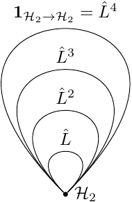
For our example we consider a 2 level atom with states \(\ket{a}\) - excited and \(\ket{b}\) - ground. As soon as we consider a 2-level system we are in the 2 dimensional Hilbert space. The category in the example will be called as \(\mathbf{Rabi}\). It has only one Object: \[\mathrm{ob}(\mathbf{Rabi}) = \{\mathcal{H}_2\}.\]
The atom interacts with light beam of frequency \(\omega = \omega_{ab}\). The state of the system is described by the following equation (Мурашко И. В. 2018): \[\ket{\psi} = \cos{\frac{\omega_R t}{2}} \ket{a} - i \sin{\frac{\omega_R t}{2}} \ket{b}, \nonumber\] where \(\omega_R\) - Rabi frequency (Мурашко И. В. 2018).
The interaction time \(t\) is fixed and corresponds to \(\omega_R t = \pi\) i.e. the interaction can be described a linear operator \(\hat{L}\).
There are 4 different Morphisms: \[\mathrm{hom}(\mathbf{Rabi}) = \{\mathbf{1}_{\mathcal{H}_2 \to \mathcal{H}_2}, \hat{L}, \hat{L}^2, \hat{L}^3\}.\] The corresponding orbit of the initial state \(\ket{\psi}_0\) is given as follows: \[\begin{aligned} \ket{\psi}_0 = \ket{a}, \nonumber \\ \ket{\psi}_1 = \hat{L} \ket{\psi}_0 = -i \ket{b}, \nonumber \\ \ket{\psi}_2 = \hat{L}^2 \ket{\psi}_0 = - \ket{a}, \nonumber \\ \ket{\psi}_3 = \hat{L}^3 \ket{\psi}_0 = i \ket{b}, \nonumber \end{aligned}\]
Categorical approach
There is an interesting relation between sets and categories. In both we consider objects(sets) and relations between them(morphisms/functions).
In the set theory we can get info about functions by looking inside the objects(sets) aka use “microscope” (Milewski 2018). For instance the definitions for Injection and Surjection are given in the terms of internal objects (sets) structure.
Contrary in the category theory we initially don’t have any info about object internal structure but can get it using the relation between the objects i.e. using Morphisms. In other words we can use “telescope” (Milewski 2018) there. For the instance in the Surjection vs Epimorphism we concluded that Epimorphism is a categorical definition for Surjection. The same conclusion for relation between Injection and Monomorphism was made in Injection vs Monomorphism.
Many constructions can be defined in the 2 different ways: via local (via “microscope”) or global (via “telescope”) approach. This gives us the following definitions.
The description of a system (object) via its relations with other systems (objects) will be called as categorical approach in the book. This description is an alternative one to an ordinary system description via its internal structure.
The opposite to Categorical approach will be called as non-categorical approach in the book. This description is an ordinary system description via its internal structure.
Categorical approach often uses so called Universal property to define different constructions. There is an informal definition of the property below
In category theory we can highlight constructions when they follow an unique pattern. There can be a lot of such constructions. We pick up the best one via a criteria that can vary for different definitions. The criteria that is used to separate a particular categorical construction from a huge amount of similar ones is called Universal property.
Typical examples of the universal property application are Product and Sum definitions. You can find the definitions later in the book (see Product and sum). The Universal property seems to be broadly used in different areas. There are several examples of such Universal property usage (see Physics) and Categorical approach (see Programming languages) below.
Programming languages
There are two basic options possible in programming language. You can use an imperative approach to implement requested functionality or declarative (functional) one. Lets illustrate it on the factorial calculation example.
The factorial can be defined in 2 forms. The first one assumes direct instruction on how to calculate it: \[n! = \prod_{i = 1}^n i,\] another one gives you a formal definition for the function: \[\begin{aligned} n! = n \cdot \left(n-1\right)!, \nonumber \\ 0! = 1 \end{aligned}\]
Straightforward approach to resolve the task is demonstrated by
C++ language in implementing (Programming languages):
int f(int n) {
  if (n < 0) {
    throw std::invalid_argument(
      "the argument has to be greater or equal 0");
  }
  int res = 1;
  for (int i = 1; i <= n; ++i) {
    res *= i;
  }
  return res;
}
The solution requires provide all details about the internal structure of the solution i.e. which variables to be used and how to calculate result using them. Thus the approach can be considered as a variation of Non-categorical approach.
Another case assume that the formal definition of the function is provided without any internal details about the implementation. I.e. the (Programming languages) is used. A functional language such as Haskell is a good candidate for the implementation:
-- Factorial
f 0 = 1
f n = n * f (n - 1)
Physics
Many physical concepts (may be every one) can be formulated in 2 ways. The first one uses differential equations (aka local approach). The second one uses integral equations (aka global approach). The first case is similar to the “microscope” usage. The second one is the similar to “telescope” approach.
Optics
Optics is another good example of Universal property in physics. In optics it can be reformulated as follows
A light beam chooses a path that requires the minimal amount of time to path through it.
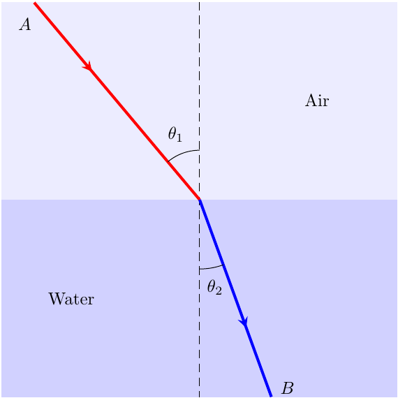
Good example of the property is shown in Optics. When the light traverse from point \(A\) to point \(B\) it does not use the shortest path because a big part of the path will be in water where speed of the light (\(v_2\)) is smaller than in air (\(v_1\)): \[v_2 < v_1\] Thus if it follows the Universal property then it should minimize the path in water that leads to well known Snell’s law (Wikipedia contributors 2019b): \[\frac{\sin \theta_2}{\sin \theta_1} = \frac{v_2}{v_1} = \frac{n_1}{n_2}.\]
Classical mechanics
we shall consider a motion of a classical mechanical system there. The system consists of \(n\) particles. Each particle with number \(i \in {1, \dots, n}\) has coordinate \(q_i \in \mathbb{R}^3\) that changes with time. The set \({q_1(t), \dots, q_n(t)}\) defines the trajectory.
Equations of classical mechanics, that define the trajectory, can be written in different forms. we shall consider Lagrangian form and least action form there. The key point for both is Lagrangian that can be written 4 as \[L = T - U,\] where \(T\) is kinetic energy and \(U\) is the potential energy. The Lagrangian is the function of particles positions \(\{q_i\}\), velocities \(\{\dot{q}_i\}\) and time \(t\). For the case of \(n\) particles we can get the following form of Lagrangian: \[L = L\left(q_1, \dots, q_n, \dot{q}_1, \dots, \dot{q}_n, t\right).\] The motion equation can be written in the following form: \[\frac{d}{dt}\left( \frac{\partial L}{\partial \dot{q}_i} \right) = \frac{\partial L}{\partial q_i}\]
Lets consider a single particle motion on the force field \(F = - \frac{d U}{d x}\). The kinetic energy is \[T = \frac{m \dot{x}^2}{2}\] and Lagrangian \[L = T - U = \frac{m \dot{x}^2}{2} - U(x).\] Thus (Classical mechanics) gives us \[\frac{d}{dt}\left( \frac{\partial L}{\partial \dot{x}} \right) = \frac{\partial L}{\partial x}\] or \[\frac{d}{dt}\left(m \dot{x}\right) = m \ddot{x} = - \frac{d U}{d x} = F\] that is the famous Newton’s second law for a particle.
The (Classical mechanics) is an example of local approach when the knowledge about local properties (this knowledge leads to the differential equation) gives us the motion equation i.e. the equation has been got using a “microscope” there.
Another way to investigate the motion is the principle of least action. In the principle we consider all possible trajectories of our system between time points \(t_1\) and \(t_2\). For each trajectory \({\bf q}(t) = {q_1(t), \dots, q_n(t)}, t \in [t_1, t_2]\) we can define the following integral \[S\left({\bf q}, t_1, t_2\right) = \int_{t_1}^{t_2}L\left({\bf q}(t), \dot{\bf q}(t), t\right) dt,\] that is called as Action. The principle of least action states that the trajectory taken by the system between times \(t_1\) and \(t_2\) is the one for which the action is stationary (no change) to first order (Wikipedia contributors 2019a) i.e. \[\delta S = 0.\] We can rewrite the principle as follows \[\begin{aligned} \delta S = \int_{t_1}^{t_2} \delta L\left({\bf q}(t), \dot{\bf q}(t), t\right) dt = \nonumber \\ = \int_{t_1}^{t_2} \left[L\left({\bf q} + \delta {\bf q} , \dot{\bf q} + \delta \dot{\bf q}, t\right) - L\left({\bf q}, \dot{\bf q}, t\right)\right] dt = \nonumber \\ = \int_{t_1}^{t_2} \left[\frac{\partial L}{\partial {\bf q}} \delta {\bf q} + \frac{\partial L}{\partial \dot{\bf q}} \delta \dot{\bf q}\right] dt = \int_{t_1}^{t_2} \frac{\partial L}{\partial {\bf q}} \delta {\bf q} dt + \nonumber \\ + \left. \frac{\partial L}{\partial \dot{\bf q}} \delta {\bf q} \right|_{t_1}^{t_2} - \int_{t_1}^{t_2} \frac{d}{d t} \left( \frac{\partial L}{\partial \dot{\bf q}} \delta {\bf q}\right) dt = \nonumber \\ = \int_{t_1}^{t_2} \left[ \frac{\partial L}{\partial {\bf q}} - \frac{d}{d t} \left( \frac{\partial L}{\partial \dot{\bf q}} \right) \right] \delta {\bf q} dt = 0, \nonumber \end{aligned}\] that leads to (Classical mechanics). Therefore the same motion equation can be used using global approach (via integral over all possible trajectories) or in other words the “telescope” was used there.
The principle of least action can be treated as an universal property that will allow to pick up one object (trajectory) among the set of the similar objects. The same universal properties will appear during the book in a lot of places.
Quantum mechanics
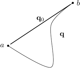
Very interesting example of Categorical approach is provided us by quantum mechanics via path integrals (Feynman, Hibbs, and Styer 2010). The question that is asked is the following. If we have 2 points \(a\) and \(b\), what’s probability \(P(a, b)\) that a particle moves from \(a\) to \(b\)? The probability is defined as follows (Feynman, Hibbs, and Styer 2010): \[P(a,b) = \left|K(a,b)\right|^2,\] where \(K(a,b)\) is a special function defined by all possible paths from \(a\) to \(b\) as follows \[K(a,b) = \frac{1}{Z} \int_{\bf q} e^{\frac{i}{\hbar}S({\bf q})} \mathcal{D}{\bf q},\] where \({\bf q}\) is a trajectory from \(a\) to \(b\) (see Quantum mechanics), and \(S\) is the action defined by (Classical mechanics). For a path \(x\) such that \(\delta S({\bf q}) > \hbar\) we shall have that a trajectory \({\bf q} + \delta {\bf q}\) that is similar to \({\bf q}\) but gives a completely different action and as result such trajectories will cancel each other.
From other hand the path \({\bf q}_0\) such that \(\delta S({\bf q}_0) = 0\) will have all other similar trajectories \({\bf q}_0 + \delta {\bf q}\) will increase each other and as result the \({\bf q}_0\) will define the real trajectory for the particle. This is in direct connection with the classical least action principle (Wikipedia contributors 2019a).
Discussion
Register with a username and password to join the discussion.