Introduction

One of the most popular public-key encryption algorithms is RSA (Rivest, Shamir, and Adleman 1978). It is built on the assumption that factorization of large integers is a difficult problem. Therefore algorithms that decompose an integer into prime factors are of special interest. Below we describe such an algorithm proposed by Shor (Shor 1994).

We will start with the classical RSA construction, because this is the place where factorization enters cryptography. After that we will reduce factorization to the problem of finding the period of a function. The quantum part of Shor’s algorithm is exactly a method for finding this period by means of the quantum Fourier transform.

The RSA Algorithm

The RSA algorithm, named after Rivest, Shamir, and Adleman, is an asymmetric encryption algorithm. In such an algorithm two different keys are used: one key encrypts the message and the other key decrypts it. The construction is based on the difficulty of decomposing a number into prime factors.

Key Generation

The key generation consists of several steps.

1. Choose two distinct prime numbers \(p\) and \(q\).

2. Compute their product \[n = p q.\]

3. Compute Euler’s function for this product: \[\varphi(n) = (p - 1)(q - 1).\]

4. Choose an integer \(e\) such that \[1 < e < \varphi(n)\] and \(e\) is coprime with \(\varphi(n)\), i.e. \[\gcd(e,\varphi(n)) = 1.\]

5. Compute \[d \equiv e^{-1} \pmod{\varphi(n)},\] or, equivalently, \[d e \equiv 1 \pmod{\varphi(n)}.\]

The public key consists of two numbers: the modulus \(n\) and the public exponent \(e\). These two numbers are used to encrypt the initial message.

The private key also consists of two numbers: the modulus \(n\) and the private exponent \(d\). The initial prime numbers \(p\) and \(q\) are kept secret, because with them the computation of \(\varphi(n)\) becomes trivial.

It is worth noting that to recover the private key from the public key one has to compute \(\varphi(n)\) from the known value of \(n\). This task is difficult if \(p\) and \(q\) are not known. Thus, knowing the factorization of \(n\) breaks the key.

Example (RSA key generation).

Let us choose two distinct prime numbers \[p = 3,\qquad q = 7.\] The product of these numbers is \[n = 21.\] Euler’s function is \[\varphi(n) = (p - 1)(q - 1) = 2 \cdot 6 = 12.\]

Now we choose the public exponent \(e\) in such a way that \(1 < e < 12\) and \[\gcd(e,12) = 1.\] Obviously \(e=5\) satisfies these conditions. The private exponent is \[d \equiv 5^{-1} \pmod{12}.\] Therefore \(d=5\). Indeed, \[5 \cdot 5 = 25 = 2 \cdot 12 + 1,\] i.e. \[5 \cdot 5 \equiv 1 \pmod{12}.\]

Thus we get

• the public key \((n=21,e=5)\);

• the private key \((n=21,d=5)\).

Encryption

Suppose that we have to encrypt a message \(M\). First it is converted to an integer, or to several integers, \(m\). For the small example below we choose \(0<m<n\). The ciphertext \(c\) is computed as follows: \[c \equiv m^e \pmod n. \label{eq:rsa-encrypt}\]

Example (RSA encryption).

Suppose that we have the public key \((n=21,e=5)\) and we want to encrypt the following message: \[m = 1101_2 = 11_{10}.\] The ciphertext is computed by formula [eq:rsa-encrypt]: \[c \equiv 11^5 \pmod {21} = 2.\]

Decryption

The message \(m\) can be recovered from \(c\) by the following formula: \[m \equiv c^d \pmod n. \label{eq:rsa-decrypt}\] Having \(m\), we can reconstruct the initial message \(M\).

Example (RSA decryption).

Suppose that we have the private key \((n=21,d=5)\) and the ciphertext \(c=2\) from the previous example. The initial text is computed by formula [eq:rsa-decrypt]: \[m \equiv 2^5 \pmod {21} = 11 = 1101_2.\]

Why Decryption Works

We want to prove that \[(m^e)^d \equiv m \pmod {p q}\] for positive integers \(m\), where \(p\) and \(q\) are distinct prime numbers, and \(e\) and \(d\) satisfy \[d e \equiv 1 \pmod{\varphi(p q)}.\] We can rewrite the last relation in the form \[d e - 1 = h(p - 1)(q - 1),\] where \(h\) is an integer. Therefore \[m^{ed} = m m^{h(p-1)(q-1)}.\]

Now there are two cases: either \(m\) is divisible by \(p\), or \(m\) and \(p\) are coprime. In the first case \[m^{ed} \equiv m \equiv 0 \pmod p.\] In the second case we use Fermat’s little theorem: \[m m^{h(p-1)(q-1)} = m \left(m^{p-1}\right)^{h(q-1)} \equiv m \cdot 1^{h(q-1)} \equiv m \pmod p.\]

Similarly, either \[m^{ed} \equiv m \equiv 0 \pmod q,\] or, by Fermat’s little theorem, \[m m^{h(p-1)(q-1)} = m \left(m^{q-1}\right)^{h(p-1)} \equiv m \cdot 1^{h(p-1)} \equiv m \pmod q.\]

Thus we have \[m^{ed} \equiv m \pmod p,\qquad m^{ed} \equiv m \pmod q.\] By the Chinese remainder theorem, \[m^{ed} \equiv m \pmod {p q}.\]

Factorization And Period Finding

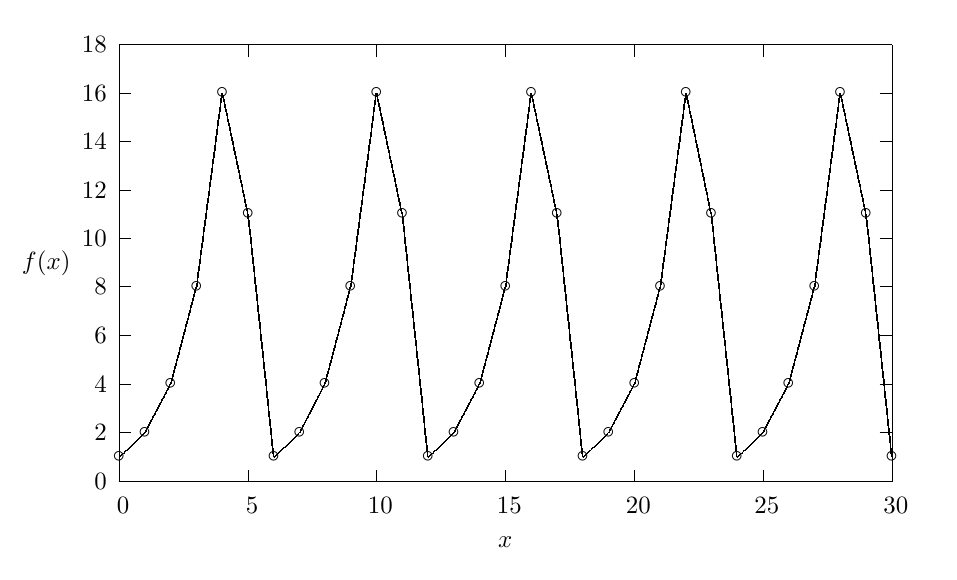
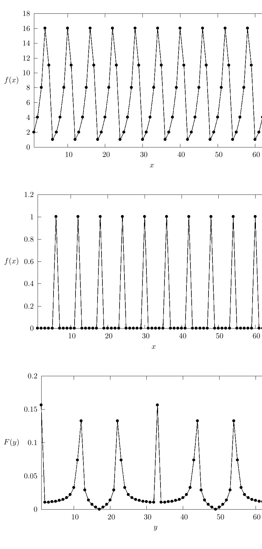
The factorization problem for an integer \(N\) is closely related to the problem of finding the period of a function. Let us consider the following function, called modular exponentiation: \[f(x,a) = a^x \bmod N. \label{eq:modular-exponentiation}\] The function [eq:modular-exponentiation] depends on the number \(N\) being analyzed and on two arguments, \(x\) and \(a\). The argument \(a\) is chosen from the following conditions: \[\begin{aligned} 0 < a < N, \nonumber \\ \gcd(N,a) = 1. \label{eq:a-conditions} \end{aligned}\]

A typical graph of this function is shown in [fig:modular-exponentiation].

The conditions [eq:a-conditions] mean that \(a\) and \(N\) do not have common divisors. If they do have such divisors, then these divisors are already the desired solution of the factorization problem and can be found by Euclid’s algorithm.

The function [eq:modular-exponentiation] is periodic, i.e. there exists a number \(r\) such that \[f(x+r,a) = f(x,a).\] The smallest possible number \(r\) is called the period of the function [eq:modular-exponentiation].

To prove periodicity, let us note that \(f(x,a)\) cannot be zero. Indeed, if \[f(x,a)=0,\] then \[\exists x\in\{0,1,\dots\}: a^x = kN,\] where \(k\) is an integer. This is impossible because \(a\) and \(N\) are coprime. Here we assume, of course, that \(N>1\).

Thus the range of [eq:modular-exponentiation] is limited by the set \[f(x,a)\in \{1,\dots,N-1\}.\] Therefore \[\exists k,j:\quad k>j,\quad k,j\in\{0,1,\dots,N\},\quad f(k,a)=f(j,a),\] which proves that the values must repeat.

Let \[k=j+r.\] Then \[a^k \bmod N = a^{j+r}\bmod N = a^j a^r \bmod N = a^j \bmod N.\] Since \(a\) and \(N\) are coprime, we can write \[a^r \equiv 1 \pmod N. \label{eq:period-condition}\]

The period of [eq:modular-exponentiation] can be even or odd. In Shor’s algorithm we are interested in the first case, an even period. Otherwise we choose a new number \(a\) and repeat the period finding step. Thus, taking \[r=2l,\] we can rewrite [eq:period-condition] as \[a^{2l}\equiv 1 \pmod N.\] At the same time, because \(r\) is the smallest number satisfying the periodicity condition, we have \[a^l \not\equiv 1 \pmod N.\] If the number \(a\) is also chosen in such a way that \[a^l \not\equiv -1 \pmod N,\] then \[(a^l-1)(a^l+1)=kN, \label{eq:factor-product}\] where \(k\) is an integer. From [eq:factor-product] we get that \(a^l-1\) and \(a^l+1\) have nontrivial common divisors with \(N\).

Example (finding divisors of \(N=21\)).

Let us consider the problem of finding divisors of \[N=21.\] Choosing \(a=2\), we get the period \[r=6\] for the function [eq:modular-exponentiation], as shown in [fig:modular-exponentiation]. Clearly, \[2^3 \equiv 8 \pmod {21} \not\equiv -1 \pmod {21}.\] Thus, by finding the corresponding greatest common divisors, we solve the factorization problem: \[\begin{aligned} \gcd(2^3-1,21) &= \gcd(7,21) = 7, \\ \gcd(2^3+1,21) &= \gcd(9,21) = 3, \\ 21 &= 7\cdot 3. \end{aligned}\]

Breaking The RSA Example

Now let us return to the RSA example. The public key was \[(n=21,e=5).\] An attacker who can factor \(n\) obtains \[21=3\cdot 7.\] After that the Euler function becomes known: \[\varphi(21)=(3-1)(7-1)=12.\] The private exponent is the inverse of \(e=5\) modulo \(12\): \[d\equiv 5^{-1}\pmod {12}=5.\] Thus the private key is recovered: \[(n=21,d=5).\] If the intercepted ciphertext is \[c=2,\] then the message is decrypted as \[m\equiv 2^5 \pmod {21}=11=1101_2.\]

Thus Shor’s algorithm does not have to decrypt RSA directly. It is enough to factor the public modulus \(n\). After factorization, the private exponent can be reconstructed by the same formula that was used in key generation.

The Shor Algorithm

Thus the factorization of \(N\) can be reduced to finding the period of a suitable function. The algorithm can be written as follows.

1. Choose a number \(a\) such that \(0<a<N\).

2. Compute \(\gcd(a,N)\). If \(\gcd(a,N)\ne 1\), then this greatest common divisor is already a nontrivial divisor of \(N\).

3. Find the period \(r\) of the function \[f(x,a)=a^x\bmod N.\]

4. If \(r\) is odd, choose a new number \(a\) and repeat the procedure.

5. If \[a^{r/2}\equiv -1\pmod N,\] choose a new number \(a\) and repeat the procedure.

6. Otherwise return \[\gcd(a^{r/2}-1,N),\qquad \gcd(a^{r/2}+1,N).\]

The classical part of this algorithm uses only arithmetic operations and the Euclidean algorithm. The difficult step is period finding. This is the place where the quantum computer is used.

Quantum Fourier Transform

For the analysis of periodic sequences and functions one can use the discrete Fourier transform. For a sequence of numbers \(\{x_m\}\) with \(M\) terms it has the form \[\tilde{X}_j = \frac{1}{\sqrt{M}}\sum_{m=0}^{M-1} x_m e^{-i\frac{2\pi}{M}jm}. \label{eq:qft-classical}\]

The quantum Fourier transform works with states of the form \[\ket{x}=\sum_{k=0}^{M-1}x_k\ket{k}, \label{eq:qft-input-series}\] where the sequence of amplitudes \(\{x_k\}\) defines the sequence for the Fourier transform [eq:qft-classical]. The basis vector \(\ket{k}\) contains the number of the corresponding term in the sequence. The amplitudes have to satisfy the normalization condition \[\sum_k |x_k|^2 = 1.\]

Suppose that an operator \(\hat{F}^M\), the quantum Fourier transform operator, acts on a basis vector according to the rule \[\hat{F}^M\ket{k} = \frac{1}{\sqrt M}\sum_{j=0}^{M-1} e^{-i\omega k j}\ket{j}_{inv}, \qquad \omega=\frac{2\pi}{M}. \label{eq:qft-basis}\] The systems of basis vectors \(\{\ket{k}\}\) and \(\{\ket{k}_{inv}\}\) are the same set of vectors, numbered in a different order. The subscript \(inv\) is used to keep this reversed order visible, as in the original circuit derivation.

From [eq:qft-input-series] and [eq:qft-basis] we get \[\begin{aligned} \hat{F}^M\ket{x} &= \sum_{k=0}^{M-1}x_k\hat{F}^M\ket{k} \nonumber \\ &= \frac{1}{\sqrt M} \sum_{k=0}^{M-1}\sum_{j=0}^{M-1} e^{-i\omega k j}x_k\ket{j}_{inv} \nonumber \\ &= \sum_{j=0}^{M-1} \left\{ \frac{1}{\sqrt M} \sum_{k=0}^{M-1}e^{-i\omega k j}x_k \right\}\ket{j}_{inv} \nonumber \\ &= \sum_{j=0}^{M-1}\tilde{X}_j\ket{j}_{inv} = \ket{\tilde{X}}_{inv}, \label{eq:qft-state-transform} \end{aligned}\] where \[\tilde{X}_j=\tilde{X}^M_j = \frac{1}{\sqrt M} \sum_{k=0}^{M-1}e^{-i\omega k j}x_k. \label{eq:qft-amplitudes}\] Thus the quantum operator repeats the classical Fourier transform on the sequence of amplitudes: \[\ket{x}\longleftrightarrow \ket{\tilde{X}}_{inv}.\]

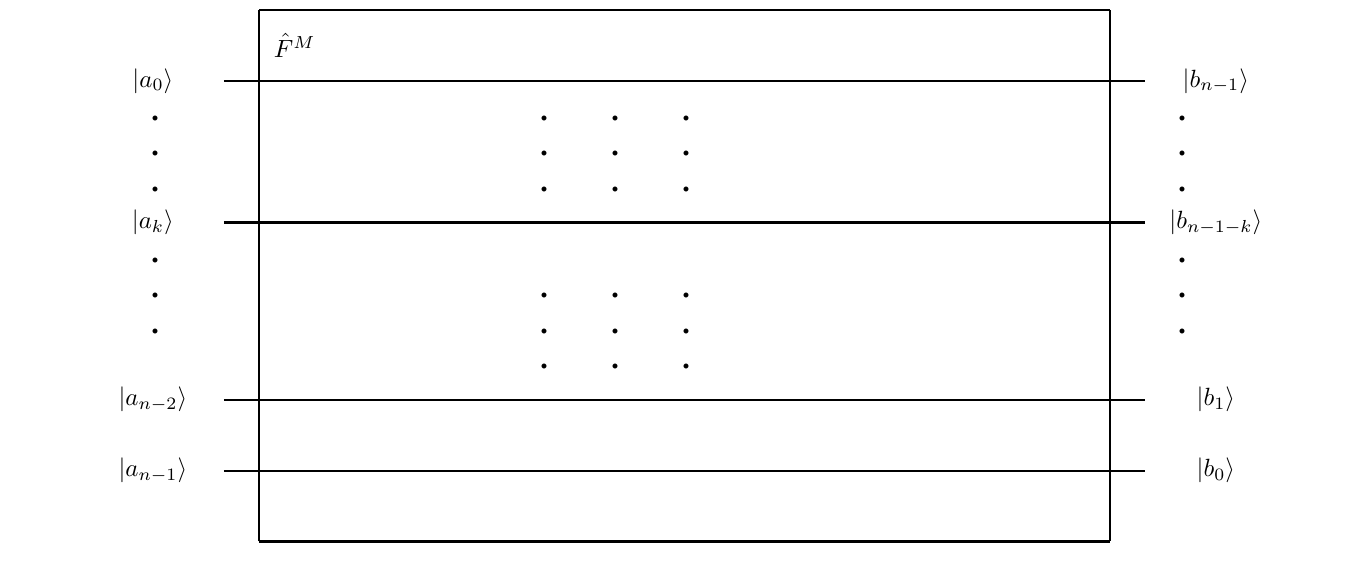
Now let us consider how this transform is implemented recursively. This derivation follows the circuit analysis from the Russian lecture notes and the corresponding paper (Murashko and Korikov 2015). Suppose that the number of basis states is a power of two: \[M=2^n.\] Then every basis state can be represented as a tensor product of \(n=\log_2 M\) qubits: \[\ket{k} = \ket{a^{(k)}_0}\otimes\ket{a^{(k)}_1} \otimes\cdots\otimes\ket{a^{(k)}_{n-1}}, \label{eq:qft-input-bits}\] where \[k=a^{(k)}_0+2a^{(k)}_1+\cdots+2^{n-1}a^{(k)}_{n-1}, \qquad a^{(k)}_i\in\{0,1\}.\] On the output we get a superposition of basis states \(\{\ket{j}_{inv}\}\), where \[\ket{j}_{inv} =\ket{b^{(j)}_{n-1}}\otimes\ket{b^{(j)}_{n-2}} \otimes\cdots\otimes\ket{b^{(j)}_0},\] and \[j=b^{(j)}_0+2b^{(j)}_1+\cdots+2^{n-1}b^{(j)}_{n-1}, \qquad b^{(j)}_i\in\{0,1\}.\]

The least significant input bit \(a^{(k)}_0\) separates the even and odd elements. Therefore the state [eq:qft-input-series] can be written as \[\begin{aligned} \ket{x} &= \sum_{m=0}^{M/2-1}x_{2m}\ket{0}\otimes\ket{m} + \sum_{m=0}^{M/2-1}x_{2m+1}\ket{1}\otimes\ket{m} \nonumber \\ &= \sum_{m=0}^{M/2-1}x_{2m}\ket{2m} + \sum_{m=0}^{M/2-1}x_{2m+1}\ket{2m+1}. \label{eq:qft-even-odd} \end{aligned}\] Here \[m=a^{(k)}_1+2a^{(k)}_2+\cdots+2^{n-2}a^{(k)}_{n-1}.\]

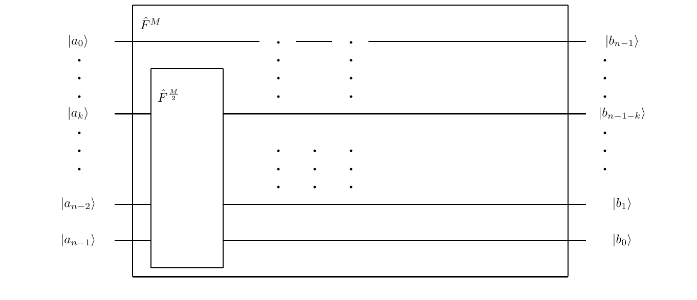
First we apply the Fourier transform only to the higher bits, i.e. we exclude \(a^{(k)}_0\). This gives \[\begin{aligned} \ket{x}\rightarrow{}& \sum_{m=0}^{M/2-1}x_{2m}\ket{0}\otimes \hat{F}^{M/2}\ket{m} +\sum_{m=0}^{M/2-1}x_{2m+1}\ket{1}\otimes \hat{F}^{M/2}\ket{m}. \label{eq:qft-step-one} \end{aligned}\] Using [eq:qft-basis] for \(\hat{F}^{M/2}\), we obtain \[\hat{F}^{M/2}\ket{m} = \sqrt{\frac{2}{M}} \sum_{j=0}^{M/2-1} e^{-i\frac{4\pi}{M}mj}\ket{j}_{inv}.\] Therefore [eq:qft-step-one] can be written in the form \[\ket{x}\rightarrow \sum_{j=0}^{M/2-1}\tilde{A}_j\ket{j}_{inv} +\sum_{j=0}^{M/2-1}\tilde{B}_j \left|\frac{M}{2}+j\right\rangle_{inv}, \label{eq:qft-ab-state}\] where \[\begin{aligned} \tilde{A}_j &= \sqrt{\frac{2}{M}} \sum_{m=0}^{M/2-1} e^{-i\frac{4\pi}{M}mj}x_{2m}, \nonumber \\ \tilde{B}_j &= \sqrt{\frac{2}{M}} \sum_{m=0}^{M/2-1} e^{-i\frac{4\pi}{M}mj}x_{2m+1}. \label{eq:qft-ab} \end{aligned}\]

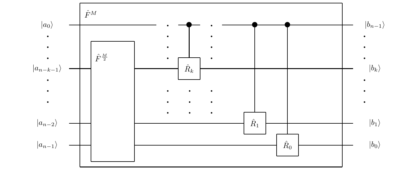
Now we add the phase shift for the odd elements, i.e. for those elements where \(a^{(k)}_0=1\). Let this phase operator be \(\hat{R}\). It acts on the state \(\left|\frac{M}{2}+j\right\rangle_{inv}\) as follows: \[\begin{aligned} \hat{R}\left|\frac{M}{2}+j\right\rangle_{inv} &= \hat{R}\ket{1}\otimes\ket{j}_{inv} \nonumber \\ &= \prod_{l=0}^{n-2} \exp\left(-2\pi i\frac{2^l b^{(j)}_l}{2^n}\right) \ket{1}\otimes\ket{j}_{inv} \nonumber \\ &= \exp\left(-2\pi i\frac{j}{M}\right) \left|\frac{M}{2}+j\right\rangle_{inv}. \label{eq:qft-phase} \end{aligned}\] In this derivation we used \[j=b^{(j)}_0+2b^{(j)}_1+\cdots+2^{n-2}b^{(j)}_{n-2}.\] Thus after the phase shift \[\tilde{C}_j = \sqrt{\frac{2}{M}} \sum_{m=0}^{M/2-1} e^{-i\frac{2\pi}{M}(2m+1)j}x_{2m+1}. \label{eq:qft-c}\]

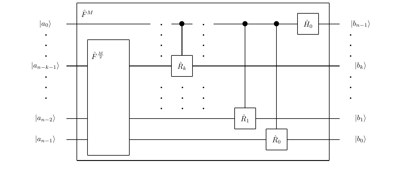
Finally we apply the Hadamard transform to the qubit \(\ket{a_0}\). We get \[\begin{aligned} \ket{x}\rightarrow{}& \sum_{j=0}^{M/2-1} \frac{\tilde{A}_j+\tilde{C}_j}{\sqrt{2}}\ket{j}_{inv} +\sum_{j=0}^{M/2-1} \frac{\tilde{A}_j-\tilde{C}_j}{\sqrt{2}} \left|\frac{M}{2}+j\right\rangle_{inv}. \label{eq:qft-step-three} \end{aligned}\] For the first group of amplitudes, using [eq:qft-ab] and [eq:qft-c], we have \[\begin{aligned} \frac{\tilde{A}_j+\tilde{C}_j}{\sqrt{2}} &= \sqrt{\frac{1}{M}} \sum_{m=0}^{M/2-1}e^{-i\frac{4\pi}{M}mj}x_{2m} +\sqrt{\frac{1}{M}} \sum_{m=0}^{M/2-1} e^{-i\frac{2\pi}{M}(2m+1)j}x_{2m+1} \nonumber \\ &= \sqrt{\frac{1}{M}} \sum_{m=0}^{M-1}e^{-i\frac{2\pi}{M}mj}x_m. \label{eq:qft-step-three-even} \end{aligned}\] For the second group, \[\begin{aligned} \frac{\tilde{A}_j-\tilde{C}_j}{\sqrt{2}} &= \sqrt{\frac{1}{M}} \sum_{m=0}^{M-1} e^{-i\frac{2\pi}{M}mj}x_m\frac{1+e^{-i\pi m}}{2} \nonumber \\ &\quad - \sqrt{\frac{1}{M}} \sum_{m=0}^{M-1} e^{-i\frac{2\pi}{M}mj}x_m\frac{1-e^{-i\pi m}}{2} \nonumber \\ &= \sqrt{\frac{1}{M}} \sum_{m=0}^{M-1} e^{-i\frac{2\pi}{M}mj}e^{-i\pi m}x_m \nonumber \\ &= \sqrt{\frac{1}{M}} \sum_{m=0}^{M-1} e^{-i\frac{2\pi}{M}m(\frac{M}{2}+j)}x_m. \label{eq:qft-step-three-odd} \end{aligned}\]

Combining [eq:qft-step-three], [eq:qft-step-three-even], and [eq:qft-step-three-odd], we finally obtain \[\begin{aligned} \ket{x}\rightarrow{}& \sum_{j=0}^{M/2-1} \sqrt{\frac{1}{M}}\sum_{m=0}^{M-1} e^{-i\frac{2\pi}{M}mj}x_m\ket{j}_{inv} \nonumber \\ &+ \sum_{j=0}^{M/2-1} \sqrt{\frac{1}{M}}\sum_{m=0}^{M-1} e^{-i\frac{2\pi}{M}m(\frac{M}{2}+j)}x_m \left|\frac{M}{2}+j\right\rangle_{inv} \nonumber \\ &= \sum_{j=0}^{M-1}\tilde{X}^M_j\ket{j}_{inv}. \label{eq:qft-final} \end{aligned}\] This is exactly the Fourier transform [eq:qft-amplitudes]. Therefore the circuit described by the successive steps above implements the quantum Fourier transform.

Period Finding By Quantum Fourier Transform

To find the period of [eq:modular-exponentiation], the circuit shown in [fig:quantum-period-finding] is used.

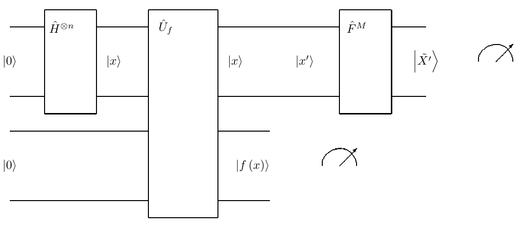
The first element is the Hadamard transform applied to \(n\) qubits. It prepares the initial state in the form \[\ket{in} = \frac{1}{\sqrt{2^n}} \sum_{x=0}^{2^n-1}\ket{x}\otimes\ket{0}.\]

After the element that computes the function, denoted by \(\hat U_f\), the state becomes \[\hat U_f\ket{in} = \frac{1}{\sqrt{2^n}} \sum_{x=0}^{2^n-1}\ket{x}\otimes\ket{f(x)}.\]

After measuring the value of the function, only those coordinates remain for which the function has the measured value. As a result, the input of the Fourier transform contains a state of the form \[\ket{in'}=\sum_{x'}\ket{x'}.\] All nonzero elements have the same amplitude and follow with the period equal to the period of the function under investigation. The initial position may have a shift that depends on the experiment. In different experiments this shift can be different. The Fourier image, however, has the same period structure for different shifts.

Therefore the most probable samples, i.e. the local maxima of the probability distribution after the Fourier transform, follow with a period related to the original period of the function. Thus, after several experiments, the required period can be found with the required probability (Nielsen and Chuang 2000).

Example (finding the period of \(f(x)=2^x\bmod 21\)).

Let us consider the problem of finding the period of \[f(x,a)=a^x\bmod N\] for \[a=2,\qquad N=21.\] The number of samples \(M\) has to be a power of two. In this example we choose \[M=2^6=64.\] Thus we need six qubits for the first register.

The initial state after the Hadamard transform is \[\ket{in} = \frac{1}{8}\sum_{x=0}^{63}\ket{x}\otimes\ket{0}.\] Here \(\ket{x}\) is the tensor product of six qubits that encode the binary representation of the function argument. For example, for \[x=5_{10}=000101_2\] we have \[\ket{x} = \ket0\otimes\ket0\otimes\ket0 \otimes\ket1\otimes\ket0\otimes\ket1.\]

After the function computation we have \[\hat U_f\ket{in} = \frac{1}{8}\sum_{x=0}^{63}\ket{x} \otimes\ket{f(x)}.\]

The original graph in [fig:shor-period-finding] uses the shifted sampling convention \(2^{x+1}\bmod 21\). This shift does not change the period. If the measured value of the function register is \(1\), then the remaining first-register state can be written in the same convention as \[\ket{in'} = \frac{1}{\sqrt{10}} \left( \ket5+\ket{11}+\ket{17}+\dots+\ket{59} \right)\otimes\ket1.\] The expression contains ten terms of equal amplitude, hence the normalizing factor is \(1/\sqrt{10}\).

The Fourier transform of this sequence is shown on the lower graph of [fig:shor-period-finding]. The most probable measurement results correspond to local maxima that repeat with period \[\frac{M}{r}\approx 10.67.\] From this we find the period of the original function: \[r=6.\]

Conclusion

The RSA example shows where the factorization problem enters public key cryptography. The public modulus \(n\) is known, but its prime factors are hidden. If these factors are found, then \(\varphi(n)\) is known, the private exponent \(d\) can be reconstructed, and the ciphertext can be decrypted.

Shor’s algorithm reduces this factorization problem to the period finding problem for the modular exponentiation function \[f(x,a)=a^x\bmod N.\] The quantum part of the algorithm prepares a periodic state and uses the quantum Fourier transform to reveal the period. Once the period is known, the factors of \(N\) are obtained by ordinary greatest common divisor computations.