Introduction

We will discuss one of the simplest places where the non-classical structure of quantum mechanics becomes visible. The objects will be photons with two orthogonal polarizations. This is a convenient model because the mathematical state space is two-dimensional, while the physical implementation still has a direct optical interpretation.

The main result of the article is the protocol of quantum teleportation. In this protocol Alice does not copy an unknown quantum state and does not send the photon itself to Bob. Instead, Alice and Bob use a previously prepared entangled pair, Alice performs a Bell-state measurement, and Bob obtains a photon whose state is related to the original state by a known local transformation (Bennett et al. 1993).

After that we will consider a second application of the same idea: the Mermin-Peres pseudo-telepathy game. In this game entanglement allows Alice and Bob to win with probability \(1\), while no classical strategy can do this (Brassard, Broadbent, and Tapp 2003; Aravind 2004).

Polarization States

Let us start with a single photon. We will use two orthogonal polarization states: \[\ket{x}, \qquad \ket{y}.\] An arbitrary pure polarization state can be written as follows: \[\ket{\psi} = \alpha\ket{x}+\beta\ket{y}, \qquad |\alpha|^2+|\beta|^2=1. \label{eq:simple-polarization-state}\] Here \(\alpha\) and \(\beta\) are complex amplitudes. The normalization condition says that a measurement in the \(\{\ket{x},\ket{y}\}\) basis gives one of the two outcomes with total probability \(1\).

It will also be useful to introduce the Stokes operators. In the single-photon subspace they are represented by the matrices \[\hat{S}_0 = \begin{pmatrix} 1 & 0 \\ 0 & 1 \end{pmatrix}, \quad \hat{S}_1 = \begin{pmatrix} 1 & 0 \\ 0 & -1 \end{pmatrix}, \quad \hat{S}_2 = \begin{pmatrix} 0 & 1 \\ 1 & 0 \end{pmatrix}, \quad \hat{S}_3 = \begin{pmatrix} 0 & i \\ -i & 0 \end{pmatrix}. \label{eq:stokes-operators}\] Each operator has eigenvalues \(\pm 1\), and \[\hat{S}_0^2=\hat{S}_1^2=\hat{S}_2^2=\hat{S}_3^2=\hat{I}.\] The operators \(\hat{S}_1,\hat{S}_2,\hat{S}_3\) are the Pauli operators up to the chosen sign convention for \(\hat{S}_3\). This minor convention will matter in the pseudo-telepathy game, where Bob will measure complex-conjugated operators.

Bell States

Now let us consider two photons. A general two-photon polarization state has the form \[\ket{\psi}_{12} = c_{xx}\ket{x}_1\ket{x}_2 + c_{xy}\ket{x}_1\ket{y}_2 + c_{yx}\ket{y}_1\ket{x}_2 + c_{yy}\ket{y}_1\ket{y}_2. \label{eq:general-two-photon-state}\] The most important two-photon states for us are the Bell states: \[\begin{aligned} \ket{\psi^{+}}_{12} &= \frac{1}{\sqrt{2}} \left( \ket{x}_1\ket{y}_2 + \ket{y}_1\ket{x}_2 \right), \nonumber \\ \ket{\psi^{-}}_{12} &= \frac{1}{\sqrt{2}} \left( \ket{x}_1\ket{y}_2 - \ket{y}_1\ket{x}_2 \right), \nonumber \\ \ket{\phi^{+}}_{12} &= \frac{1}{\sqrt{2}} \left( \ket{x}_1\ket{x}_2 + \ket{y}_1\ket{y}_2 \right), \nonumber \\ \ket{\phi^{-}}_{12} &= \frac{1}{\sqrt{2}} \left( \ket{x}_1\ket{x}_2 - \ket{y}_1\ket{y}_2 \right). \label{eq:bell-basis} \end{aligned}\] These states form an orthonormal basis in the two-photon polarization space. For example, if we write them in the basis \[\ket{x}_1\ket{x}_2,\quad \ket{x}_1\ket{y}_2,\quad \ket{y}_1\ket{x}_2,\quad \ket{y}_1\ket{y}_2,\] then \[\ket{\psi^{+}}_{12} = \frac{1}{\sqrt{2}} \begin{pmatrix} 0 \\ 1 \\ 1 \\ 0 \end{pmatrix}, \qquad \ket{\psi^{-}}_{12} = \frac{1}{\sqrt{2}} \begin{pmatrix} 0 \\ 1 \\ -1 \\ 0 \end{pmatrix}.\] Therefore \[\braket{\psi^{+}}{\psi^{-}} = \frac{1}{2} \begin{pmatrix} 0 & 1 & 1 & 0 \end{pmatrix} \begin{pmatrix} 0 \\ 1 \\ -1 \\ 0 \end{pmatrix} = \frac{1}{2}(1-1) =0.\] The other scalar products are checked in the same way. Thus every state of the form [eq:general-two-photon-state] can be expanded in the Bell basis.

Generation and Registration

Entangled photon pairs can be obtained by spontaneous parametric down-conversion. In the type-II phase matching case the two photons have different polarizations and propagate along two cones. The schematic geometry is shown in Figure 1.

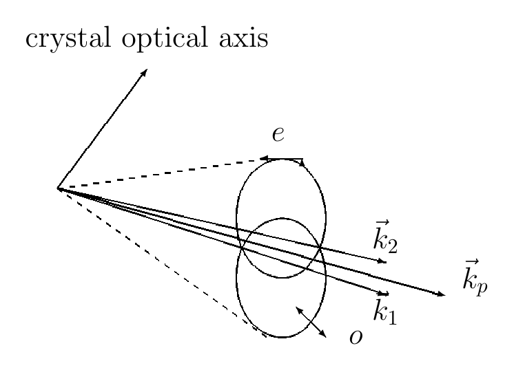
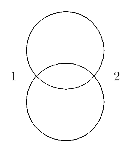
If we look in the directions where the two cones intersect, then the state can be written as follows: \[\ket{\psi} = \frac{1}{\sqrt{2}} \left( \ket{x}_1\ket{y}_2 + e^{i\alpha}\ket{y}_1\ket{x}_2 \right), \label{eq:down-conversion-state}\] where \(\alpha\) is the phase difference between the ordinary and extraordinary rays. By adding a birefringent plate one can choose \(\alpha=0\) or \(\alpha=\pi\). Therefore the same setup can produce \(\ket{\psi^{+}}_{12}\) and \(\ket{\psi^{-}}_{12}\). The two intersection directions are shown schematically in Figure 2.

The states \(\ket{\phi^{+}}_{12}\) and \(\ket{\phi^{-}}_{12}\) are obtained from these states by placing a half-wave plate in one of the beams: \[\ket{x}\longrightarrow\ket{y}, \qquad \ket{y}\longrightarrow\ket{x}.\] Thus the four Bell states form not only a useful mathematical basis, but also a physically accessible family of polarization states.

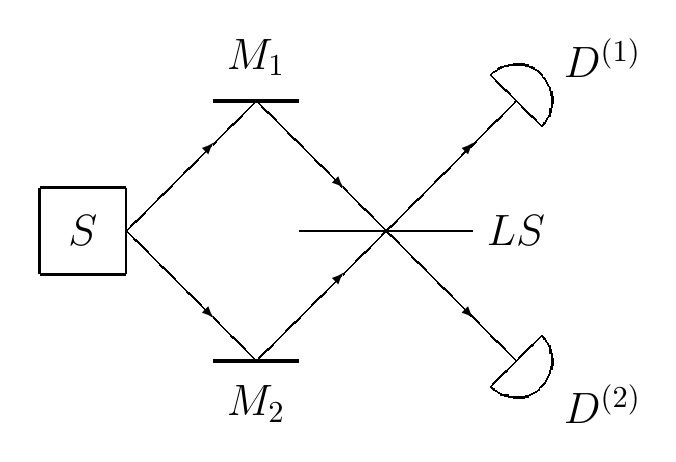
The next question is how to detect a Bell state. The simplest case is the antisymmetric state \(\ket{\psi^{-}}_{12}\). It can be separated from the other three states by sending two photons to a beam splitter, as shown in Figure 3.

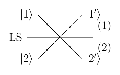
The beam splitter acts on the spatial modes as a Hadamard transformation: \[\begin{aligned} \hat{H}\ket{1} &= \frac{1}{\sqrt{2}} \left(\ket{1'}+\ket{2'}\right), \nonumber \\ \hat{H}\ket{2} &= \frac{1}{\sqrt{2}} \left(\ket{1'}-\ket{2'}\right). \label{eq:beam-splitter-hadamard} \end{aligned}\] The action is shown in Figure 4.

There are two possible spatial states for a pair of photons entering the beam splitter from opposite sides: \[\begin{aligned} \ket{S}_{12} &= \frac{1}{\sqrt{2}} \left( \ket{1}_1\ket{2}_2 + \ket{2}_1\ket{1}_2 \right), \nonumber \\ \ket{A}_{12} &= \frac{1}{\sqrt{2}} \left( \ket{1}_1\ket{2}_2 - \ket{2}_1\ket{1}_2 \right). \label{eq:spatial-symmetric-antisymmetric} \end{aligned}\] The state \(\ket{S}_{12}\) is symmetric under exchange of the two photons, while \(\ket{A}_{12}\) is antisymmetric.

Let us transform the symmetric state. Using [eq:beam-splitter-hadamard], we obtain \[\begin{aligned} \hat{H}\ket{S}_{12} &= \frac{1}{\sqrt{2}} \left( \hat{H}\ket{1}_1\hat{H}\ket{2}_2 + \hat{H}\ket{2}_1\hat{H}\ket{1}_2 \right) \nonumber \\ &= \frac{1}{2\sqrt{2}} \left( (\ket{1'}_1+\ket{2'}_1)(\ket{1'}_2-\ket{2'}_2) \right. \nonumber \\ &\qquad\left. +(\ket{1'}_1-\ket{2'}_1)(\ket{1'}_2+\ket{2'}_2) \right) \nonumber \\ &= \frac{1}{\sqrt{2}} \left( \ket{1'}_1\ket{1'}_2 - \ket{2'}_1\ket{2'}_2 \right). \label{eq:beam-splitter-symmetric} \end{aligned}\] Both photons leave through the same output side. For the antisymmetric spatial state we get the opposite result: \[\begin{aligned} \hat{H}\ket{A}_{12} &= \frac{1}{\sqrt{2}} \left( \hat{H}\ket{1}_1\hat{H}\ket{2}_2 - \hat{H}\ket{2}_1\hat{H}\ket{1}_2 \right) \nonumber \\ &= -\frac{1}{\sqrt{2}} \left( \ket{1'}_1\ket{2'}_2 - \ket{2'}_1\ket{1'}_2 \right). \label{eq:beam-splitter-antisymmetric} \end{aligned}\] In this case the two photons leave through different output sides.

Photons are bosons, so the total wave function, including polarization and spatial parts, must be symmetric. Therefore the antisymmetric polarization state \(\ket{\psi^{-}}_{12}\) must be paired with the antisymmetric spatial state. This is why a coincidence click in the two detectors identifies \(\ket{\psi^{-}}_{12}\).

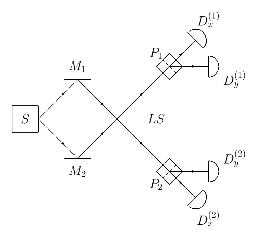
In a polarization-resolving version of the same registration scheme, each output beam is split by a Nicol prism and then sent to two detectors, as shown in Figure 5.

No-Cloning

Before discussing teleportation, we have to state a limitation. An unknown quantum state cannot be cloned (Wootters and Zurek 1982). Suppose that there is a device with an initial state \(\ket{D_I}\) and a cloning operator \(\hat{D}\). If the input photon is in the state \(\ket{x}\), then the device should produce two copies: \[\hat{D}\ket{D_I}\ket{x} = \ket{D_{F_x}}\ket{x}\ket{x}.\] For the state \(\ket{y}\) we similarly have \[\hat{D}\ket{D_I}\ket{y} = \ket{D_{F_y}}\ket{y}\ket{y}.\] Now let us apply the same operator to the arbitrary state [eq:simple-polarization-state]. By linearity, \[\begin{aligned} \hat{D}\ket{D_I} \left( \alpha\ket{x}+\beta\ket{y} \right) &= \alpha\ket{D_{F_x}}\ket{x}\ket{x} + \beta\ket{D_{F_y}}\ket{y}\ket{y}. \label{eq:no-cloning-linearity} \end{aligned}\] This is not the same as the desired cloned state \[\ket{D_F} \left( \alpha\ket{x}+\beta\ket{y} \right) \left( \alpha\ket{x}+\beta\ket{y} \right). \label{eq:no-cloning-desired}\] Indeed, [eq:no-cloning-desired] contains the cross terms \(\alpha\beta\ket{x}\ket{y}\) and \(\alpha\beta\ket{y}\ket{x}\), while [eq:no-cloning-linearity] does not. Thus a universal cloning device is impossible.

Teleportation does not contradict this theorem. The original state is destroyed by Alice’s measurement, and Bob receives only one instance of the state.

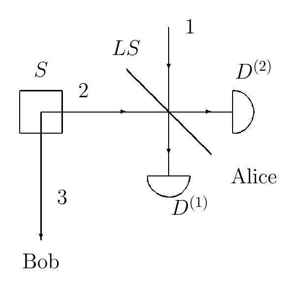
Quantum Teleportation

The optical teleportation scheme is shown in Figure 6. Alice wants to send Bob the unknown state of photon \(1\): \[\ket{\psi}_1 = \alpha\ket{x}_1+\beta\ket{y}_1. \label{eq:teleported-state}\] In addition, Alice and Bob share an entangled pair of photons \(2\) and \(3\): \[\ket{\psi^{-}}_{23} = \frac{1}{\sqrt{2}} \left( \ket{x}_2\ket{y}_3 - \ket{y}_2\ket{x}_3 \right). \label{eq:teleportation-pair}\] Photon \(2\) is sent to Alice, and photon \(3\) is sent to Bob.

The state of the full three-photon system is \[\ket{\Psi}_{123} = \ket{\psi}_1\ket{\psi^{-}}_{23}. \label{eq:three-photon-state}\] We have to rewrite this state in the Bell basis of photons \(1\) and \(2\). The useful inverse relations are \[\begin{aligned} \ket{x}_1\ket{x}_2 &= \frac{1}{\sqrt{2}} \left(\ket{\phi^{+}}_{12}+\ket{\phi^{-}}_{12}\right), \nonumber \\ \ket{y}_1\ket{y}_2 &= \frac{1}{\sqrt{2}} \left(\ket{\phi^{+}}_{12}-\ket{\phi^{-}}_{12}\right), \nonumber \\ \ket{x}_1\ket{y}_2 &= \frac{1}{\sqrt{2}} \left(\ket{\psi^{+}}_{12}+\ket{\psi^{-}}_{12}\right), \nonumber \\ \ket{y}_1\ket{x}_2 &= \frac{1}{\sqrt{2}} \left(\ket{\psi^{+}}_{12}-\ket{\psi^{-}}_{12}\right). \label{eq:bell-inverse-relations} \end{aligned}\] Substituting [eq:teleported-state] and [eq:teleportation-pair] into [eq:three-photon-state], we obtain \[\begin{aligned} \ket{\Psi}_{123} &= \frac{1}{\sqrt{2}} \left( \alpha\ket{x}_1\ket{x}_2\ket{y}_3 - \alpha\ket{x}_1\ket{y}_2\ket{x}_3 \right. \nonumber \\ &\qquad\left. + \beta\ket{y}_1\ket{x}_2\ket{y}_3 - \beta\ket{y}_1\ket{y}_2\ket{x}_3 \right) \nonumber \\ &= \frac{1}{2}\ket{\psi^{+}}_{12} \left( -\alpha\ket{x}_3+\beta\ket{y}_3 \right) \nonumber \\ &\quad -\frac{1}{2}\ket{\psi^{-}}_{12} \left( \alpha\ket{x}_3+\beta\ket{y}_3 \right) \nonumber \\ &\quad +\frac{1}{2}\ket{\phi^{+}}_{12} \left( -\beta\ket{x}_3+\alpha\ket{y}_3 \right) \nonumber \\ &\quad +\frac{1}{2}\ket{\phi^{-}}_{12} \left( \beta\ket{x}_3+\alpha\ket{y}_3 \right). \label{eq:teleportation-bell-expansion} \end{aligned}\] The most important term for the optical scheme above is the term with \(\ket{\psi^{-}}_{12}\). We can also find it directly by projection: \[\begin{aligned} \bra{\psi^{-}}_{12}\ket{\Psi}_{123} &= \frac{1}{\sqrt{2}} \left( \bra{x}_1\bra{y}_2 - \bra{y}_1\bra{x}_2 \right) \nonumber \\ &\quad \times \left( \alpha\ket{x}_1+\beta\ket{y}_1 \right) \frac{1}{\sqrt{2}} \left( \ket{x}_2\ket{y}_3 - \ket{y}_2\ket{x}_3 \right) \nonumber \\ &= \frac{1}{2} \left( \alpha\bra{y}_2-\beta\bra{x}_2 \right) \left( \ket{x}_2\ket{y}_3 - \ket{y}_2\ket{x}_3 \right) \nonumber \\ &= -\frac{1}{2} \left( \alpha\ket{x}_3+\beta\ket{y}_3 \right). \label{eq:teleportation-projection} \end{aligned}\] The factor \(-1/2\) consists of a probability amplitude and a global phase. The physical state of Bob’s photon is the same as the original state [eq:teleported-state].

Therefore, every time Alice detects photons \(1\) and \(2\) in the Bell state \(\ket{\psi^{-}}_{12}\), Bob’s photon is in the state \[\alpha\ket{x}_3+\beta\ket{y}_3.\] This is the teleportation event. In a complete Bell-state measurement one can also use the other three outcomes; Bob then applies the corresponding local correction. Experiments with complete Bell-state measurement for polarization teleportation were demonstrated in (Kim, Kulik, and Shih 2001).

It is worth noting what is and is not transmitted. No material photon travels from Alice to Bob. Also, Alice’s measurement result must be communicated through an ordinary classical channel, so the protocol does not allow faster-than-light communication.

The Mermin-Peres Game

Entanglement also gives a clean example where quantum correlations win a game that has no perfect classical strategy. We will use the Mermin-Peres square, which is one of the standard pseudo-telepathy examples.

The game is played by Alice and Bob against a referee. Alice receives the number of a row in a \(3\times 3\) square. Bob receives the number of a column. Alice must fill her row with numbers \(\pm 1\), and Bob must fill his column with numbers \(\pm 1\). Alice’s row must have product \(+1\), while Bob’s column must have product \(-1\). They win if their numbers agree at the intersection of Alice’s row and Bob’s column.

Example.

Suppose that Alice receives row \(1\), and Bob receives column \(3\). One winning pair of answers is \[A = \begin{pmatrix} +1 & -1 & -1 \\ * & * & * \\ * & * & * \end{pmatrix}, \qquad B = \begin{pmatrix} * & * & -1 \\ * & * & +1 \\ * & * & +1 \end{pmatrix}.\] The row product is \(+1\), the column product is \(-1\), and both players write \(-1\) in the common entry.

The players may agree on a strategy before the round starts, but after they receive the row and column numbers they are isolated from each other.

No Classical Perfect Strategy

Classically, a perfect strategy would mean that Alice and Bob have implicitly agreed on all nine entries of one square. This is impossible. If all rows have product \(+1\), then the product of all nine entries, computed row by row, is \[(+1)(+1)(+1)=+1.\] On the other hand, if all columns have product \(-1\), then the product of the same nine entries, computed column by column, is \[(-1)(-1)(-1)=-1.\] The same product cannot be both \(+1\) and \(-1\). Thus every classical strategy must fail for at least one choice of row and column.

Quantum Strategy

Now suppose that before the game starts Alice and Bob prepare two maximally entangled pairs: \[\ket{\Omega} = \ket{\Phi^{+}}_{A_1B_1} \otimes \ket{\Phi^{+}}_{A_2B_2}, \qquad \ket{\Phi^{+}}_{AB} = \frac{1}{\sqrt{2}} \left( \ket{x}_A\ket{x}_B + \ket{y}_A\ket{y}_B \right). \label{eq:magic-square-state}\] Alice keeps photons \(A_1,A_2\), and Bob keeps photons \(B_1,B_2\).

Consider the following matrix of two-photon observables: \[X = \begin{pmatrix} \hat{S}_0\otimes\hat{S}_3 & \hat{S}_3\otimes\hat{S}_0 & \hat{S}_3\otimes\hat{S}_3 \\ \hat{S}_1\otimes\hat{S}_0 & \hat{S}_0\otimes\hat{S}_1 & \hat{S}_1\otimes\hat{S}_1 \\ -\hat{S}_1\otimes\hat{S}_3 & -\hat{S}_3\otimes\hat{S}_1 & \hat{S}_2\otimes\hat{S}_2 \end{pmatrix}. \label{eq:magic-square-operators}\] Denote the entries of this matrix by \(\hat{x}_{ij}\). Each entry satisfies \[\hat{x}_{ij}^2=\hat{I}.\] Therefore each measurement gives one of the two values \(\pm 1\).

Alice uses the matrix \(X\). If she receives row \(i\), she jointly measures the three commuting operators in that row and writes the three obtained eigenvalues. Bob uses the complex-conjugated matrix \(X^*\). If he receives column \(j\), he jointly measures the three commuting operators in that column and writes the three obtained eigenvalues.

The conjugation in Bob’s measurements is only a convention issue. With our choice \[\hat{S}_3 = \begin{pmatrix} 0 & i \\ -i & 0 \end{pmatrix},\] we have \(\hat{S}_3^*=-\hat{S}_3\). This is why the correlation identity below uses \(\hat{x}_{ij}^*\) on Bob’s side.

Let us verify the parity conditions. The product of the first row is \[(\hat{S}_0\otimes\hat{S}_3) (\hat{S}_3\otimes\hat{S}_0) (\hat{S}_3\otimes\hat{S}_3) = \hat{S}_3^2\otimes\hat{S}_3^2 = \hat{I}.\] The second row is similar: \[(\hat{S}_1\otimes\hat{S}_0) (\hat{S}_0\otimes\hat{S}_1) (\hat{S}_1\otimes\hat{S}_1) = \hat{S}_1^2\otimes\hat{S}_1^2 = \hat{I}.\] For the third row we use the multiplication relations between the Stokes operators. From [eq:stokes-operators] one checks that \[\hat{S}_1\hat{S}_3=i\hat{S}_2, \qquad \hat{S}_3\hat{S}_1=-i\hat{S}_2.\] Therefore \[\begin{aligned} &(-\hat{S}_1\otimes\hat{S}_3) (-\hat{S}_3\otimes\hat{S}_1) (\hat{S}_2\otimes\hat{S}_2) \nonumber \\ &\quad = (\hat{S}_1\hat{S}_3\hat{S}_2) \otimes (\hat{S}_3\hat{S}_1\hat{S}_2) \nonumber \\ &\quad = (i\hat{S}_2^2)\otimes(-i\hat{S}_2^2) = \hat{I}. \label{eq:magic-square-third-row} \end{aligned}\] Thus the product of Alice’s row is always \(+1\).

Now consider the columns. For the first column, \[(\hat{S}_0\otimes\hat{S}_3) (\hat{S}_1\otimes\hat{S}_0) (-\hat{S}_1\otimes\hat{S}_3) = -\hat{S}_1^2\otimes\hat{S}_3^2 = -\hat{I}.\] The second column gives the same result. For the third column, \[\begin{aligned} &(\hat{S}_3\otimes\hat{S}_3) (\hat{S}_1\otimes\hat{S}_1) (\hat{S}_2\otimes\hat{S}_2) \nonumber \\ &\quad = (\hat{S}_3\hat{S}_1\hat{S}_2) \otimes (\hat{S}_3\hat{S}_1\hat{S}_2) \nonumber \\ &\quad = (-i\hat{I})\otimes(-i\hat{I}) = -\hat{I}. \label{eq:magic-square-third-column} \end{aligned}\] Complex conjugation preserves these products, so Bob’s measured column also has product \(-1\).

It remains to prove that Alice and Bob obtain the same value at the intersection. We will use the following property of the maximally entangled state: \[\left(\hat{M}\otimes\hat{M}^{*}\right)\ket{\Phi^{+}} = \ket{\Phi^{+}} \label{eq:maximal-entanglement-correlation}\] for every unitary one-qubit operator \(\hat{M}\) satisfying \(\hat{M}^2=\hat{I}\). Indeed, if \(\hat{M}\ket{x}=m_{xx}\ket{x}+m_{yx}\ket{y}\) and \(\hat{M}\ket{y}=m_{xy}\ket{x}+m_{yy}\ket{y}\), then applying \(\hat{M}\otimes\hat{M}^*\) to \(\ket{\Phi^+}\) gives \[\frac{1}{\sqrt{2}} \sum_{a,b,c\in\{x,y\}} m_{ba}m^*_{ca}\ket{b}\ket{c} = \frac{1}{\sqrt{2}} \sum_{b,c\in\{x,y\}} (\hat{M}\hat{M}^{\dagger})_{bc}\ket{b}\ket{c} = \ket{\Phi^+}.\] The same argument applies to products of two such operators. Hence, for every entry of [eq:magic-square-operators], \[\left( \hat{x}_{ij} \otimes \hat{x}_{ij}^{*} \right) \ket{\Omega} = \ket{\Omega}. \label{eq:magic-square-intersection}\] This means that the product of Alice’s and Bob’s measurement results at the same position is always \(+1\). Since both values are either \(+1\) or \(-1\), they must be equal.

Therefore Alice and Bob satisfy all three requirements in every round. Classically they cannot preassign all nine numbers without contradiction. Quantum mechanically they do not preassign all nine numbers at once; instead they measure only one commuting row or one commuting column, and the entangled state guarantees agreement at the shared entry.

Conclusion

Entanglement makes the state of a composite system more than a list of states of its parts. In teleportation, this allows Alice and Bob to transfer an unknown polarization state without cloning it. In the Mermin-Peres game, the same kind of non-classical correlation gives a perfect winning strategy where every classical strategy must sometimes fail.

Both examples also show the same limitation. Entanglement by itself is not a communication channel. Alice and Bob still need an ordinary classical channel to compare or use the measurement outcomes.