Introduction

From the moment when information became important, methods for protecting it started to appear. One of the simplest examples is the Caesar cipher: each letter is replaced by another letter, shifted by a fixed number of positions in the alphabet. Such a method can be broken by using the statistical properties of the language in which the message is written.

Historically, the security of a cipher often depended on keeping the algorithm secret. Modern classical cryptography usually follows a different principle. The algorithm is public and can be studied by anyone. The secret part is a key, which is mixed with the message by an open algorithm.

We will start with this classical model. It leads to a clear result: there exists an absolutely secure classical encryption scheme, the one-time pad. But the same result also exposes the main practical problem. Alice and Bob must first obtain the same random key, and the key must be as long as the message. Quantum cryptography does not replace encryption by magic. It addresses this missing step: it gives Alice and Bob a physical way to distribute a key and to test whether Eve has interfered with the source.

Classical Encryption Model

Suppose Alice wants to send a digital message to Bob. Let \(P\) denote the plaintext, \(K\) the secret key, and \(C\) the ciphertext. The encryption algorithm \(E\) transforms the plaintext and the key into the ciphertext: \[E_K(P)=C. \label{eq:classical-encryption}\] After that \(C\) is sent to Bob. Bob uses the decryption algorithm \(D\) and the same key \(K\) to recover the original message: \[D_K(C)=P. \label{eq:classical-decryption}\]

This simple scheme separates three questions.

1. How can Alice and Bob obtain a common secret key?

2. Does there exist an encryption algorithm that is absolutely secure once the key is shared?

3. Can Alice and Bob detect listening or substitution on the channel used for distributing the key?

Classical cryptography gives a precise answer to the second question. An absolutely secure cipher exists. It is the one-time pad.

One-Time Pad

The one-time pad uses a random key of the same length as the message, and this key is used only once. In the form associated with Vernam’s telegraph cipher, encryption is a symbol-by-symbol modular addition (Vernam 1926).

Suppose the alphabet contains \(X\) symbols. For the English alphabet, if we ignore punctuation and case, we can take \(X=26\) and encode letters as follows: \[A\mapsto 0,\qquad B\mapsto 1,\qquad \ldots,\qquad Z\mapsto 25.\] The \(i\)-th symbol is encrypted by \[C_i = E_{K_i}(P_i)=P_i+K_i \pmod X, \label{eq:one-time-pad-modular-encryption}\] and decrypted by \[P_i = D_{K_i}(C_i)=C_i-K_i \pmod X. \label{eq:one-time-pad-modular-decryption}\] Here \(P_i\), \(K_i\), and \(C_i\) are the plaintext, key, and ciphertext symbols at position \(i\).

For binary data the same construction uses XOR: \[0\oplus 0=0,\qquad 0\oplus 1=1,\qquad 1\oplus 0=1,\qquad 1\oplus 1=0.\] Thus \[C_i=P_i\oplus K_i, \qquad P_i=C_i\oplus K_i. \label{eq:one-time-pad-xor}\]

Claude Shannon proved that this scheme is perfectly secure if the key is truly random, has the same length as the message, and is never reused (Shannon 1949). We can state the condition as follows. A cipher is perfectly secure if, for any two messages \(m_0\) and \(m_1\) of the same length and for any ciphertext \(c\), \[P(E_K(m_0)=c)=P(E_K(m_1)=c), \label{eq:perfect-security}\] where \(K\) is chosen uniformly at random from the set of all possible keys.

For the one-time pad this follows immediately. For a fixed ciphertext \(c\) and a fixed message \(m\), the key is determined uniquely: \[k=c\oplus m. \label{eq:one-time-pad-unique-key}\] Therefore, if all keys of length \(l\) are equally likely, then \[P(E_K(m_0)=c) = P(E_K(m_1)=c) = \frac{1}{|K|}.\] The ciphertext statistics do not distinguish \(m_0\) from \(m_1\). Thus the ciphertext gives Eve no information about the plaintext.

The Key-Distribution Problem

If the one-time pad is perfectly secure, then what is wrong with classical cryptography? The problem is not the encryption step. The problem is the key.

Alice and Bob need a key that satisfies three conditions:

• the key has the same length as the message;

• the key is random;

• the key is never used twice.

Large random keys are difficult to generate and, more importantly, difficult to distribute. If Alice sends the key to Bob through the same channel that Eve can observe, then the perfect secrecy of the one-time pad has not helped. The message is protected only after the key has already been shared.

Classical public-key cryptography is the usual way to solve this problem in practice. In such systems Alice publishes an encryption key and keeps a private decryption key. Bob can encrypt a shared session key with Alice’s public key, and Alice can recover it with her private key. This idea is the foundation of modern public-key cryptography (Diffie and Hellman 1976; Rivest, Shamir, and Adleman 1978).

The price is that the security is computational. For example, RSA is based on the difficulty of factoring large integers. This difficulty is not a theorem that forbids fast algorithms. It is an assumption about what classical algorithms can do efficiently. Moreover, Shor’s quantum algorithm factors integers and computes discrete logarithms in time polynomial in the input size (Shor 1994). Thus a sufficiently large fault-tolerant quantum computer would attack the mathematical assumption behind RSA.

This is the point where quantum cryptography enters the discussion. It does not make the one-time pad unnecessary. On the contrary, it tries to create the kind of shared random key that the one-time pad requires.

Entangled Photons

We will consider a key-distribution scheme based on entangled photon pairs and a Bell test. The underlying physical state is \[\ket{\psi} = \frac{ \ket{x}_1\ket{y}_2 - \ket{y}_1\ket{x}_2 }{\sqrt{2}}, \label{eq:bell-singlet-state}\] where \(\ket{x}\) and \(\ket{y}\) are two orthogonal photon polarizations. Photon \(1\) is sent to Alice, and photon \(2\) is sent to Bob.

We will use the following Stokes observables. Alice randomly measures one of two quantities: \[\hat{A}=\hat{S}^{(1)}_1, \qquad \hat{A}'=\hat{S}^{(1)}_2.\] Bob randomly measures one of four quantities: \[\begin{aligned} \hat{B} &= \frac{1}{\sqrt{2}} \left(\hat{S}^{(2)}_1+\hat{S}^{(2)}_2\right), \nonumber \\ \hat{B}' &= \frac{1}{\sqrt{2}} \left(\hat{S}^{(2)}_1-\hat{S}^{(2)}_2\right), \nonumber \\ \hat{C} &= \hat{S}^{(2)}_1, \nonumber \\ \hat{C}' &= \hat{S}^{(2)}_2. \label{eq:bob-observables} \end{aligned}\] Each measurement gives one of the two values \(+1\) or \(-1\).

The state [eq:bell-singlet-state] has anti-correlations in the same polarization basis. Therefore, when Alice measures \(\hat{A}\) and Bob measures \(\hat{C}\), their results are opposite. The same is true for the pair \(\hat{A}'\), \(\hat{C}'\). These anti-correlated results can be converted into common random bits by flipping one side.

Bell-Test Key Distribution

The key-distribution scheme is shown in Figure 1.

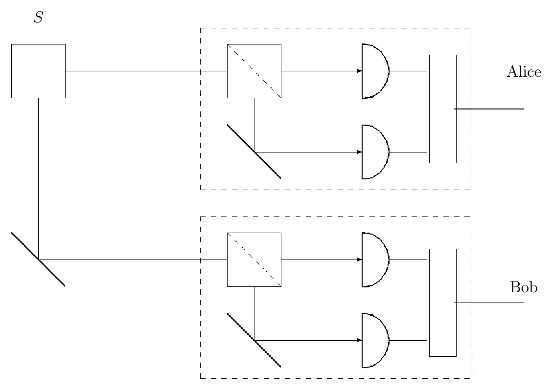
The protocol has the following form.

1. The source \(S\) emits pairs of entangled photons in the state [eq:bell-singlet-state].

2. Alice randomly chooses between \(\hat{A}\) and \(\hat{A}'\).

3. Bob randomly chooses among \(\hat{B}\), \(\hat{B}'\), \(\hat{C}\), and \(\hat{C}'\).

4. After many trials Alice and Bob announce, over a public channel, which observables they measured in each trial. They do not announce the measurement results that may become key bits.

5. In this idealized version of the protocol, trials in which a photon was not registered are discarded. This assumes that the detected subset is a fair sample of the emitted pairs.

6. The pairs \((A,C)\) and \((A',C')\) are used to form the raw key. Since the results are anti-correlated, one side flips its bits.

7. The pairs \((A,B)\), \((A',B)\), \((A,B')\), and \((A',B')\) are published and used to test a Bell inequality.

8. The remaining pairs \((A,C')\) and \((A',C)\) are discarded.

Thus the same experiment produces two kinds of data. Some trials become secret key bits. Other trials are deliberately revealed and used to check whether the photon pairs behaved as entangled quantum systems. In a practical device-independent implementation the losses cannot simply be ignored: no-detection events have to be included in the Bell test or removed by a loophole-closing setup. The simplified protocol below keeps the same fair-sampling idealization as the lecture source.

The Bell Test

In one trial Alice measures only one of the observables \(\hat{A}\), \(\hat{A}'\), and Bob measures only one of the observables \(\hat{B}\), \(\hat{B}'\), \(\hat{C}\), \(\hat{C}'\). Therefore the Bell-test value is not computed from four outcomes obtained in the same trial. It is computed from four groups of trials.

Let \[E(A,B),\qquad E(A',B),\qquad E(A,B'),\qquad E(A',B')\] denote the empirical averages of the products of the corresponding published outcomes. Then Alice and Bob estimate \[\langle F\rangle_N = \frac{1}{2} \left( E(A,B) + E(A',B) + E(A,B') - E(A',B') \right). \label{eq:bell-test-average}\] For a large number of trials this empirical value approaches the corresponding expectation value \(\langle F\rangle\).

The quantum prediction for the entangled state [eq:bell-singlet-state] is \[\begin{aligned} \langle F\rangle_{\text{quant}} &= \frac{1}{2} \bra{\psi} \left( \hat{A}\hat{B} + \hat{A}'\hat{B} + \hat{A}\hat{B}' - \hat{A}'\hat{B}' \right) \ket{\psi} \nonumber \\ &= \frac{1}{2} \bra{\psi} \left( \hat{A}(\hat{B}+\hat{B}') + \hat{A}'(\hat{B}-\hat{B}') \right) \ket{\psi} \nonumber \\ &= \frac{1}{\sqrt{2}} \bra{\psi} \left( \hat{S}^{(1)}_1\hat{S}^{(2)}_1 + \hat{S}^{(1)}_2\hat{S}^{(2)}_2 \right) \ket{\psi} \nonumber \\ &= \frac{1}{\sqrt{2}}(-1-1) = -\sqrt{2}. \label{eq:bell-quantum-value} \end{aligned}\]

Now compare this with a classical hidden-variable description. In such a description the source prepares photons with predetermined values \[a,\qquad a',\qquad b,\qquad b',\] each equal to \(+1\) or \(-1\). Then the same expression becomes \[\begin{aligned} f(a,a',b,b') &= \frac{1}{2} \left( ab+a'b+ab'-a'b' \right) \nonumber \\ &= \frac{1}{2} \left( a(b+b')+a'(b-b') \right). \label{eq:bell-classical-function} \end{aligned}\] There are two cases. If \(b=b'\), then \[f=\frac{1}{2}(2ab)=\pm 1.\] If \(b=-b'\), then \[f=\frac{1}{2}(2a'b)=\pm 1.\] Thus a classical predetermined-source model can only give \[-1\le \langle F\rangle_{\text{class}}\le 1. \label{eq:bell-classical-bound}\] The quantum value \(-\sqrt{2}\) is outside this interval. This is the Bell-inequality violation (Bell 1964; Freedman and Clauser 1972).

Detecting Eve

Suppose Eve wants to learn the key. One possible attack is to replace the entangled source by her own source. She sends Alice and Bob photons with predetermined polarization properties, and she tries to know in advance what the results of their measurements will be.

But then the measurement data are described by classical values \(a,a',b,b'\). In that case the published Bell-test trials must satisfy [eq:bell-classical-bound]. Alice and Bob compare the observed \(\langle F\rangle\) with the quantum value [eq:bell-quantum-value]. If the value is not close to the quantum prediction, they reject the key as compromised.

This is the central difference from ordinary classical key exchange. The security check is not only a statement about the complexity of a mathematical problem. It is a test of the physical correlations in the systems that generated the key. This is the idea behind entanglement-based quantum cryptography (Ekert 1991).

The Public Channel Still Matters

There is an important limitation. Alice and Bob must still use a public classical channel to compare their measurement settings and to publish the Bell-test subset. This channel does not need to be secret, but it must be authenticated.

If the public channel is not authenticated, Eve can attempt a man-in-the-middle attack. She can pretend to be Bob when talking to Alice and pretend to be Alice when talking to Bob. Then Alice and Bob would not be checking the same experiment against each other. They would each be checking an experiment controlled by Eve.

Thus quantum key distribution solves the problem in a precise sense. It does not eliminate the need for all classical assumptions. Instead, it replaces a computational assumption about factoring or discrete logarithms with a physical test of entanglement, together with the ordinary requirement that the public discussion channel is authentic.

Conclusion

Classical cryptography already contains an ideal encryption method: the one-time pad. Its weakness is practical rather than logical. Alice and Bob need a long, random, never-reused common key.

Public-key cryptography gives a practical classical answer, but its security rests on assumptions about computational hardness. Quantum computing changes this landscape because algorithms such as Shor’s attack the number-theoretic problems used by common public-key systems.

Quantum cryptography based on entanglement addresses the key distribution problem from another direction. Alice and Bob use entangled photon pairs to create correlated random data. They sacrifice part of the data to test a Bell inequality. If the test gives the quantum value, the remaining correlated data can be used as a key. If Eve replaces the source by a classical predetermined one, the Bell-test value moves into the classical interval and the key is rejected.