Introduction

Classical light is not simply light of high intensity. A laser beam can be weak and still have statistical properties that are well described by a classical random electromagnetic field. On the other hand, a field state can be bright and still have no classical probabilistic description. The difference is not in the size of the signal, but in the structure of its fluctuations.

We will study one of the simplest ways to see this difference. The observable quantity is the second-order coherence function, measured by correlating photon counts at two detectors. For many classical sources photons tend to arrive in groups. For coherent light the arrivals are Poissonian. For some quantum sources the opposite effect is possible: after one photon is detected, the probability of detecting another photon immediately after it is reduced. This is photon antibunching.

The goal of this article is to derive the basic criterion \[g^{(2)}(0) < 1\] and to explain why it is a sign of nonclassical light. The derivation will use only the photon-number operator, the variance of photon counts, and the coherent-state representation of a density matrix.

Second-Order Coherence

Let us consider a single mode of the electromagnetic field. We denote the annihilation and creation operators by \(\hat{a}\) and \(\hat{a}^{\dagger}\). They satisfy the commutation relation \[\left[\hat{a},\hat{a}^{\dagger}\right]=1.\] The photon-number operator is \[\hat{n}=\hat{a}^{\dagger}\hat{a}.\]

The normalized second-order coherence at zero delay is defined as \[g^{(2)}(0)= \frac{ \left\langle \hat{a}^{\dagger}\hat{a}^{\dagger}\hat{a}\hat{a} \right\rangle }{ \left\langle \hat{a}^{\dagger}\hat{a} \right\rangle^2 }. \label{eq:second-order-coherence}\] This expression appears naturally in delayed-coincidence measurements: the numerator counts pairs of detection events, while the denominator normalizes the result by the square of the mean intensity. We assume that \(\langle \hat{n} \rangle > 0\), so that the normalization is well-defined.

It is useful to rewrite this definition through the photon-number operator. Since \[\hat{a}^{\dagger}\hat{a}^{\dagger}\hat{a}\hat{a} = \hat{a}^{\dagger}\hat{a} \left(\hat{a}^{\dagger}\hat{a}-1\right) = \hat{n}\left(\hat{n}-1\right),\] we obtain \[g^{(2)}(0) = \frac{\left\langle \hat{n}^2 \right\rangle -\left\langle \hat{n} \right\rangle} {\left\langle \hat{n} \right\rangle^2}. \label{eq:g2-number}\] Thus the second-order coherence is a statement about the statistics of photon counts.

The Classical Bound

Now let us compare this quantum expression with the classical description. In a classical single-mode field the complex amplitude is a number \(\alpha\), and the intensity is \[I=\left|\alpha\right|^2.\] The field can fluctuate, so we describe it by an ordinary positive probability distribution over amplitudes. In that case the classical second-order coherence is \[g_{\mathrm{cl}}^{(2)}(0) = \frac{\left\langle I^2\right\rangle} {\left\langle I\right\rangle^2}. \label{eq:g2-classical}\]

From this expression we immediately get a restriction. Consider \[\begin{aligned} g_{\mathrm{cl}}^{(2)}(0)-1 &= \frac{\left\langle I^2\right\rangle} {\left\langle I\right\rangle^2} -1 \nonumber \\ &= \frac{\left\langle I^2\right\rangle -\left\langle I\right\rangle^2} {\left\langle I\right\rangle^2} \nonumber \\ &= \frac{\left\langle \left(I-\left\langle I\right\rangle\right)^2 \right\rangle} {\left\langle I\right\rangle^2} \ge 0. \label{eq:classical-bound} \end{aligned}\] The last inequality is just positivity of the variance. Therefore any classical field described by a positive probability distribution of intensities satisfies \[g_{\mathrm{cl}}^{(2)}(0) \ge 1. \label{eq:g2-classical-bound}\]

This is the first important result. If an optical field has \(g^{(2)}(0)<1\), then its photon-counting statistics cannot be explained by such a classical random intensity.

Photon Statistics

We can make the criterion more explicit by introducing the variance of the photon number, \[\operatorname{Var}(n) = \left\langle \hat{n}^2 \right\rangle -\left\langle \hat{n} \right\rangle^2.\] Substituting this into the photon-number expression for \(g^{(2)}(0)\), we obtain \[\begin{aligned} g^{(2)}(0) &= \frac{\left\langle \hat{n}^2 \right\rangle -\left\langle \hat{n} \right\rangle} {\left\langle \hat{n} \right\rangle^2} \nonumber \\ &= 1+ \frac{ \operatorname{Var}(n)-\left\langle \hat{n}\right\rangle }{ \left\langle \hat{n}\right\rangle^2 }. \label{eq:g2-variance} \end{aligned}\]

The last formula shows how the photon statistics control the second-order coherence. For a Poisson distribution we have \[\operatorname{Var}(n)=\left\langle \hat{n}\right\rangle,\] and therefore \(g^{(2)}(0)=1\). This is the photon-counting behavior of a coherent state.

If \[\operatorname{Var}(n)<\left\langle \hat{n}\right\rangle,\] then the photon stream is more regular than a Poisson stream. This is called sub-Poissonian light. In this case \[g^{(2)}(0)<1,\] and the field is nonclassical. The experimentally observed antibunching of resonance fluorescence is a standard example of this behavior (Kimble, Dagenais, and Mandel 1977). Mandel’s analysis of resonance fluorescence gives the corresponding sub-Poissonian photon statistics (Mandel 1979).

If \[\operatorname{Var}(n)>\left\langle \hat{n}\right\rangle,\] then the photon stream is less regular than a Poisson stream. This is called super-Poissonian light and corresponds to photon bunching.

The same classification is often expressed through the Fano factor \[F=\frac{\operatorname{Var}(n)}{\left\langle \hat{n}\right\rangle}.\] Then \[g^{(2)}(0)-1 = \frac{F-1}{\left\langle \hat{n}\right\rangle}. \label{eq:g2-fano}\] Thus \(F<1\) is equivalent to \(g^{(2)}(0)<1\).

Hanbury Brown-Twiss Measurement

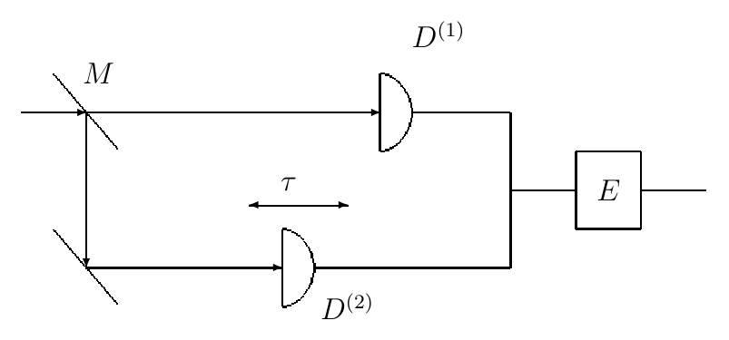
The quantity \(g^{(2)}\) is measured by a delayed-coincidence experiment. The historical starting point is the Hanbury Brown-Twiss intensity interferometer (Hanbury Brown and Twiss 1956). In a laboratory version of this measurement, a light beam is split by a half-silvered mirror and sent to two photodetectors. The electronics counts how often the two detectors click with a time delay \(\tau\).

The measured function is the normalized delayed correlation \[g^{(2)}(\tau) = \frac{\left\langle I(t) I(t+\tau)\right\rangle} {\left\langle I(t)\right\rangle^2}\] in a classical description, or the corresponding normally ordered operator expression in the quantum description (Glauber 1963b). For large \(\tau\), the two detection events become independent and the normalized correlation tends to one. The interesting behavior is near \(\tau=0\).

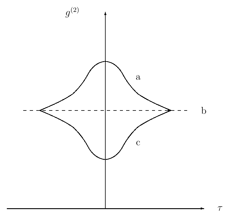
For bunched light the function has a maximum near zero delay. This means that the detection of one photon increases the probability of detecting another photon soon after it. For Poissonian light the normalized correlation is flat. For antibunched light the function has a minimum at zero delay. This means that immediately after one photon has been detected, the probability of a second detection is suppressed.

This last behavior is impossible for a classical field with a positive intensity distribution, because it gives \(g^{(2)}(0)<1\). Thus the HBT experiment turns the abstract inequality \(g^{(2)}(0)\ge 1\) into an experimentally accessible test.

The Positive P-Function Criterion

There is another way to state the same conclusion. Coherent states give a bridge between classical fields and quantum fields. Glauber and Sudarshan showed that the density operator of a field can be represented in the form \[\hat{\rho} = \int P(\alpha) \left|\alpha\right\rangle \left\langle\alpha\right| d^2\alpha, \label{eq:p-representation}\] where \(P(\alpha)\) is the Glauber-Sudarshan \(P\) function (Glauber 1963a; Sudarshan 1963). If \(P(\alpha)\) is a positive ordinary probability density, then the field behaves classically for all normally ordered measurements.

Let us apply this representation to the nonclassicality criterion. For normally ordered products we have \[\begin{aligned} \left\langle \hat{a}^{\dagger}\hat{a}^{\dagger}\hat{a}\hat{a} \right\rangle &= \int P(\alpha) \left|\alpha\right|^4 d^2\alpha, \nonumber \\ \left\langle \hat{n}\right\rangle &= \int P(\alpha) \left|\alpha\right|^2 d^2\alpha. \label{eq:p-normal-ordering} \end{aligned}\]

Suppose \(P(\alpha)\) is positive. Then the following integral must be nonnegative: \[\begin{aligned} \int P(\alpha) \left(\left|\alpha\right|^2-\left\langle \hat{n}\right\rangle\right)^2 d^2\alpha &\ge 0. \label{eq:p-positive} \end{aligned}\] Expanding the square gives \[\begin{aligned} &\int P(\alpha) \left(\left|\alpha\right|^2-\left\langle \hat{n}\right\rangle\right)^2 d^2\alpha \nonumber \\ &= \int P(\alpha)\left|\alpha\right|^4 d^2\alpha -2\left\langle \hat{n}\right\rangle \int P(\alpha)\left|\alpha\right|^2 d^2\alpha +\left\langle \hat{n}\right\rangle^2 \int P(\alpha)d^2\alpha \nonumber \\ &= \left\langle \hat{a}^{\dagger}\hat{a}^{\dagger}\hat{a}\hat{a} \right\rangle -\left\langle \hat{n}\right\rangle^2. \label{eq:p-positive-expanded} \end{aligned}\] Therefore positive \(P(\alpha)\) implies \[\left\langle \hat{a}^{\dagger}\hat{a}^{\dagger}\hat{a}\hat{a} \right\rangle \ge \left\langle \hat{n}\right\rangle^2,\] or equivalently \(g^{(2)}(0)\ge 1\).

If an experiment gives \(g^{(2)}(0)<1\), then the final expression above is negative. This contradicts the assumption that \(P(\alpha)\) is a positive probability density. Hence the \(P\) function must fail to be positive, or must be more singular than an ordinary probability density. This is why the Glauber-Sudarshan representation gives a precise mathematical meaning to the phrase nonclassical light (Klyshko 1996).

Conclusion

The second-order coherence function separates several familiar types of light by their photon-counting statistics. Coherent light has \(g^{(2)}(0)=1\). Bunched light has \(g^{(2)}(0)>1\). Antibunched light has \(g^{(2)}(0)<1\).

The last case is the essential one. In a classical field theory with a positive probability distribution of intensities, the inequality \(g^{(2)}(0)\ge 1\) follows from the positivity of variance. In quantum optics the same quantity can be smaller than one because the field operators do not behave like commuting classical amplitudes. The photon stream can be more regular than a Poisson stream, and immediately successive detections can be suppressed.

Thus photon antibunching and sub-Poissonian statistics give a direct operational criterion for nonclassical light. The same criterion is visible in the coherent-state representation: a field with \(g^{(2)}(0)<1\) cannot be represented by a positive Glauber-Sudarshan \(P(\alpha)\) distribution.