Introduction

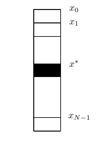
Let us consider the following problem. Suppose that we have a large set of data consisting of \(N\) elements, and we have to find an element that satisfies some condition. Schematically this problem is shown in Figure 1.

If the data are sorted, then algorithms of the “divide and conquer” type can find the required element in time of order \(O(\log N)\). In many cases the initial data set cannot be prepared for such a fast search. In this case the classical search is performed in time of order \(O(N)\).

One example is a symmetric encryption algorithm where the task is to determine the key from a known ciphertext and the corresponding plaintext. In this case preliminary preparation of the data is not available, and the direct solution of the problem is a simple search over all possible values.

Grover’s algorithm (Grover 1996) solves the problem of unstructured search in time of order \(O(\sqrt{N})\).

The Oracle

Suppose that we have a quantum circuit which computes the value of a function \(f(x)\). This function can take only two values, \(0\) and \(1\). The value \(1\) corresponds only to the element that we are looking for: \[\begin{aligned} \left.f(x)\right|_{x=x^\ast} &= 1, \\ \left.f(x)\right|_{x\ne x^\ast} &= 0. \end{aligned} \label{eq:grover-function}\] Here and below we assume that there is one marked element \(x^\ast\).

Figure 2 shows a circuit that computes this function. At the output we have a state of the form \[\ket{out} = \frac{1}{\sqrt{N}} \left( \sum_{x\ne x^\ast}\ket{x}\otimes\ket{0} + \ket{x^\ast}\otimes\ket{1} \right), \label{eq:grover-direct-output}\] where \(N\) is the total number of elements in the sequence where the search is performed.

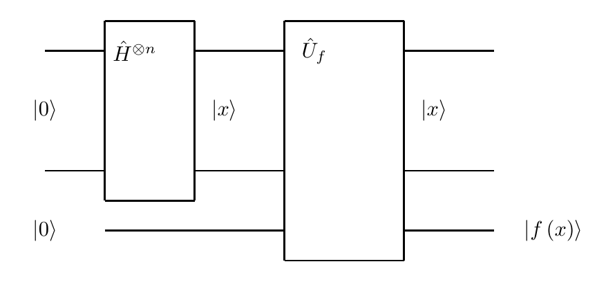
If we look at [eq:grover-direct-output], we can see that this scheme computes the function at the required point, but it still does not allow us to choose the required element. All elements in the resulting sequence are equally probable. In other words, each element can be selected by measurement with probability \(1/N\).

Grover proposed an algorithm which increases the probability of detecting the required element in the resulting superposition.

Grover Iteration

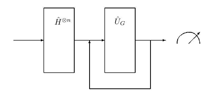
The circuit that implements Grover’s algorithm consists of a block described by an operator \(\hat{U}_G\). This block is repeated a certain number of times, as shown in Figure 3. At each iteration the probability of detecting the required element increases.

The basic element \(\hat{U}_G\) is the sequential action of two operators, as shown in Figure 4: \[\hat{U}_G = \hat{U}_s\hat{U}_{x^\ast}, \label{eq:grover-block}\] where \(\hat{U}_{x^\ast}\) is the phase inversion operator, and \(\hat{U}_s\) is the operator of inversion about the mean.

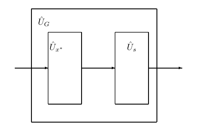
The most important point is that the two operators in [eq:grover-block] do not directly reveal \(x^\ast\). Instead, they change the amplitudes so that the amplitude of \(\ket{x^\ast}\) becomes larger than the amplitudes of the other basis states.

Phase Inversion

The action of the operator \(\hat{U}_{x^\ast}\) is described by the following relation: \[\hat{U}_{x^\ast} \left(\sum_x \alpha_x \ket{x}\right) = \sum_x \alpha_x (-1)^{f(x)}\ket{x}. \label{eq:grover-phase-inversion}\] Thus the marked state changes its sign, while all other basis states remain unchanged. Figure 5 shows this operation schematically.

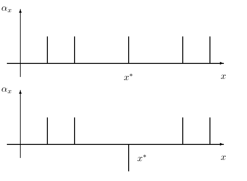
The operator \(\hat{U}_{x^\ast}\) can be rewritten as follows: \[\hat{U}_{x^\ast} = \hat{I} - 2\ket{x^\ast}\left\langle x^\ast\right|. \label{eq:grover-phase-projector}\] Indeed, we have \[\begin{aligned} &\left(\hat{I} - 2\ket{x^\ast}\left\langle x^\ast\right|\right) \left(\sum_x \alpha_x \ket{x}\right) \nonumber \\ &\quad = \sum_x \alpha_x\ket{x} - 2\alpha_{x^\ast}\ket{x^\ast} \nonumber \\ &\quad = \sum_{x\ne x^\ast}\alpha_x\ket{x} - \alpha_{x^\ast}\ket{x^\ast} \nonumber \\ &\quad = \sum_x \alpha_x(-1)^{f(x)}\ket{x}, \label{eq:grover-phase-projector-check} \end{aligned}\] which coincides with [eq:grover-phase-inversion].

Now let us discuss how this phase inversion can be implemented. In other words, we have to understand how the value \(f(x)\) can be sent into the phase.

Consider the circuit shown in Figure 6. It performs the transformation \[\ket{x}\otimes\ket{b} \longrightarrow \ket{x}\otimes\ket{b\oplus f(x)}, \label{eq:grover-oracle-action}\] where \[a\oplus b = a + b \mod 2.\]

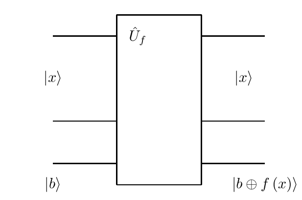
For the case \[\ket{b} = \ket{-} = \frac{\ket{0}-\ket{1}}{\sqrt{2}},\] we obtain two cases. If \(x\ne x^\ast\), then \(f(x)=0\), and \[\begin{aligned} \ket{x}\otimes\ket{-} &\longrightarrow \ket{x}\otimes \left( \frac{\ket{0\oplus 0}-\ket{1\oplus 0}}{\sqrt{2}} \right) \nonumber \\ &= \ket{x}\otimes \left( \frac{\ket{0}-\ket{1}}{\sqrt{2}} \right) \nonumber \\ &= \ket{x}\otimes\ket{-}. \label{eq:grover-phase-kickback-zero} \end{aligned}\] If \(x=x^\ast\), then \(f(x)=1\), and \[\begin{aligned} \ket{x}\otimes\ket{-} &\longrightarrow \ket{x}\otimes \left( \frac{\ket{0\oplus 1}-\ket{1\oplus 1}}{\sqrt{2}} \right) \nonumber \\ &= \ket{x}\otimes \left( \frac{\ket{1}-\ket{0}}{\sqrt{2}} \right) \nonumber \\ &= -\ket{x}\otimes\ket{-}. \label{eq:grover-phase-kickback-one} \end{aligned}\] Therefore we have the transformation \[\ket{x}\otimes\ket{-} \longrightarrow (-1)^{f(x)}\ket{x}\otimes\ket{-}. \label{eq:grover-phase-kickback-result}\] This is exactly the phase inversion from [eq:grover-phase-inversion]; the auxiliary qubit remains in the state \(\ket{-}\).

Inversion About the Mean

The action of the operator \(\hat{U}_s\) is described by the following relation: \[\hat{U}_s \left(\sum_x \alpha_x\ket{x}\right) = \sum_x (2\mathcal{M}-\alpha_x)\ket{x}, \label{eq:grover-mean-inversion}\] where \[\mathcal{M} = \frac{1}{N}\sum_x \alpha_x.\] This operation is shown schematically in Figure 7.

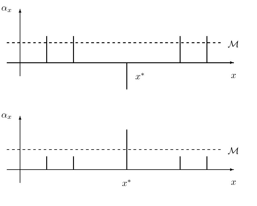
The operator \(\hat{U}_s\) can be rewritten in the following form: \[\hat{U}_s = 2\ket{s}\left\langle s\right| - \hat{I}, \label{eq:grover-mean-projector}\] where \[\ket{s} = \frac{1}{\sqrt{N}}\sum_x \ket{x}\] is the initial state in Grover’s algorithm. Indeed, \[\begin{aligned} &\left(2\ket{s}\left\langle s\right|-\hat{I}\right) \left(\sum_x \alpha_x\ket{x}\right) \nonumber \\ &\quad = 2\sum_x \alpha_x\left\langle s\middle|x\right\rangle\ket{s} -\sum_x \alpha_x\ket{x} \nonumber \\ &\quad = \frac{2}{N}\sum_x \alpha_x\sum_x\ket{x} -\sum_x\alpha_x\ket{x} \nonumber \\ &\quad = \sum_x (2\mathcal{M}-\alpha_x)\ket{x}, \label{eq:grover-mean-projector-check} \end{aligned}\] which coincides with [eq:grover-mean-inversion].

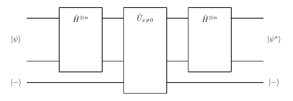
It remains to show how this operator can be realized. Consider the circuit shown in Figure 8. The element \(\hat{U}_{x\ne 0}\) performs a transformation analogous to [eq:grover-phase-kickback-result], but now the function is defined by \[f(x=0)=0,\qquad f(x\ne 0)=1.\] Thus \[\begin{aligned} \hat{U}_{x\ne 0}\ket{x}\otimes\ket{-} &= \ket{x}\otimes\ket{-}, && x=0, \nonumber \\ \hat{U}_{x\ne 0}\ket{x}\otimes\ket{-} &= -\ket{x}\otimes\ket{-}, && x\ne 0. \label{eq:grover-nonzero-action} \end{aligned}\]

If we omit the unchanged auxiliary state \(\ket{-}\), the matrix of this transformation on the search register has the form \[\begin{aligned} \hat{U}_{x\ne 0} &= \begin{pmatrix} 1 & 0 & 0 & \cdots & 0 \\ 0 & -1 & 0 & \cdots & 0 \\ 0 & 0 & -1 & \cdots & 0 \\ \vdots & \vdots & \vdots & \ddots & \vdots \\ 0 & 0 & 0 & \cdots & -1 \end{pmatrix} \nonumber \\ &= \begin{pmatrix} 2 & 0 & 0 & \cdots & 0 \\ 0 & 0 & 0 & \cdots & 0 \\ 0 & 0 & 0 & \cdots & 0 \\ \vdots & \vdots & \vdots & \ddots & \vdots \\ 0 & 0 & 0 & \cdots & 0 \end{pmatrix} - \begin{pmatrix} 1 & 0 & 0 & \cdots & 0 \\ 0 & 1 & 0 & \cdots & 0 \\ 0 & 0 & 1 & \cdots & 0 \\ \vdots & \vdots & \vdots & \ddots & \vdots \\ 0 & 0 & 0 & \cdots & 1 \end{pmatrix}. \label{eq:grover-nonzero-matrix} \end{aligned}\]

Combining this result with two Hadamard transformations, and using \[\hat{H}^{\otimes n}\ket{0} = \frac{1}{\sqrt{N}}\sum_x\ket{x} = \ket{s}, \qquad N=2^n,\] we obtain \[\begin{aligned} &\hat{H}^{\otimes n} \left\{ \begin{pmatrix} 2 & 0 & 0 & \cdots & 0 \\ 0 & 0 & 0 & \cdots & 0 \\ 0 & 0 & 0 & \cdots & 0 \\ \vdots & \vdots & \vdots & \ddots & \vdots \\ 0 & 0 & 0 & \cdots & 0 \end{pmatrix} - \hat{I} \right\} \hat{H}^{\otimes n} \nonumber \\ &\quad = \left\{ \begin{pmatrix} \frac{2}{N} & \frac{2}{N} & \frac{2}{N} & \cdots & \frac{2}{N} \\ \frac{2}{N} & \frac{2}{N} & \frac{2}{N} & \cdots & \frac{2}{N} \\ \frac{2}{N} & \frac{2}{N} & \frac{2}{N} & \cdots & \frac{2}{N} \\ \vdots & \vdots & \vdots & \ddots & \vdots \\ \frac{2}{N} & \frac{2}{N} & \frac{2}{N} & \cdots & \frac{2}{N} \end{pmatrix} - \hat{I} \right\} \nonumber \\ &\quad = \begin{pmatrix} \frac{2}{N}-1 & \frac{2}{N} & \frac{2}{N} & \cdots & \frac{2}{N} \\ \frac{2}{N} & \frac{2}{N}-1 & \frac{2}{N} & \cdots & \frac{2}{N} \\ \frac{2}{N} & \frac{2}{N} & \frac{2}{N}-1 & \cdots & \frac{2}{N} \\ \vdots & \vdots & \vdots & \ddots & \vdots \\ \frac{2}{N} & \frac{2}{N} & \frac{2}{N} & \cdots & \frac{2}{N}-1 \end{pmatrix}. \label{eq:grover-mean-implementation-matrix} \end{aligned}\]

If we act by the operator \(\hat{H}^{\otimes n}\hat{U}_{x\ne 0}\hat{H}^{\otimes n}\), then from [eq:grover-mean-implementation-matrix] we obtain \[\begin{aligned} &\hat{H}^{\otimes n}\hat{U}_{x\ne 0}\hat{H}^{\otimes n} \sum_x\alpha_x\ket{x} \nonumber \\ &\quad = \begin{pmatrix} \frac{2}{N}-1 & \frac{2}{N} & \frac{2}{N} & \cdots & \frac{2}{N} \\ \frac{2}{N} & \frac{2}{N}-1 & \frac{2}{N} & \cdots & \frac{2}{N} \\ \frac{2}{N} & \frac{2}{N} & \frac{2}{N}-1 & \cdots & \frac{2}{N} \\ \vdots & \vdots & \vdots & \ddots & \vdots \\ \frac{2}{N} & \frac{2}{N} & \frac{2}{N} & \cdots & \frac{2}{N}-1 \end{pmatrix} \begin{pmatrix} \alpha_0 \\ \alpha_1 \\ \alpha_2 \\ \vdots \\ \alpha_{N-1} \end{pmatrix} \nonumber \\ &\quad = \begin{pmatrix} \frac{2}{N}\sum_x\alpha_x-\alpha_0 \\ \frac{2}{N}\sum_x\alpha_x-\alpha_1 \\ \frac{2}{N}\sum_x\alpha_x-\alpha_2 \\ \vdots \\ \frac{2}{N}\sum_x\alpha_x-\alpha_{N-1} \end{pmatrix} \nonumber \\ &\quad = \sum_x(2\mathcal{M}-\alpha_x)\ket{x}. \label{eq:grover-mean-implementation-check} \end{aligned}\] Therefore the circuit from Figure 8 does implement inversion about the mean.

Number of Iterations

The schematic form of Grover’s algorithm can be written as follows.

1. Prepare the initial state \[\ket{\psi}_0 \Leftarrow \frac{1}{\sqrt{N}}\sum_x\ket{x}.\]

2. Repeat \[\ket{\psi}_t \Leftarrow \hat{U}_s\hat{U}_{x^\ast}\ket{\psi}_{t-1}\] until \(t\) reaches approximately \[\frac{\pi}{4}\sqrt{N}.\]

3. Measure the state \(\ket{\psi}_t\).

We are interested in two questions. What is the algorithmic complexity of Grover’s algorithm? And do there exist algorithms that can perform the search in an unstructured volume of data more efficiently than Grover’s algorithm?

The criterion of efficiency is the following fact: a good algorithm has to find the required value with the minimal number of calls to the function [eq:grover-function].

Let us consider the first iteration. The initial state \(\ket{\psi}_0\) has the following form: \[\ket{\psi}_0 = \sum_x\alpha_x\ket{x} = \ket{s} = \frac{1}{\sqrt{N}}\sum_x\ket{x} = \frac{1}{\sqrt{N}}\sum_{x\ne x^\ast}\ket{x} + \frac{1}{\sqrt{N}}\ket{x^\ast}. \label{eq:grover-initial-state}\] Thus the coefficient before the required element is \[\alpha_{x^\ast} = \frac{1}{\sqrt{N}}.\]

After applying the phase inversion operator \(\hat{U}_{x^\ast}\) from [eq:grover-phase-inversion], we obtain \[\hat{U}_{x^\ast}\ket{\psi}_0 = \frac{1}{\sqrt{N}}\sum_{x\ne x^\ast}\ket{x} - \frac{1}{\sqrt{N}}\ket{x^\ast} = \sum_x\beta_x\ket{x}, \label{eq:grover-after-phase}\] where \[\beta_{x^\ast} = -\frac{1}{\sqrt{N}}, \qquad \beta_{x\ne x^\ast} = \frac{1}{\sqrt{N}}.\]

After applying the inversion-about-the-mean operator \(\hat{U}_s\) from [eq:grover-mean-inversion], we obtain \[\begin{aligned} \hat{U}_G\ket{\psi}_0 &= \hat{U}_s\hat{U}_{x^\ast}\ket{\psi}_0 = \hat{U}_s\sum_x\beta_x\ket{x} \nonumber \\ &= \sum_x(2\mathcal{M}-\beta_x)\ket{x} \nonumber \\ &\approx \sum_{x\ne x^\ast} \left( 2\frac{1}{\sqrt{N}}-\frac{1}{\sqrt{N}} \right) \ket{x} + \left( 2\frac{1}{\sqrt{N}}+\frac{1}{\sqrt{N}} \right) \ket{x^\ast} \nonumber \\ &= \frac{1}{\sqrt{N}}\sum_{x\ne x^\ast}\ket{x} + \frac{3}{\sqrt{N}}\ket{x^\ast}. \label{eq:grover-first-rough} \end{aligned}\] In the derivation of [eq:grover-first-rough] we used the approximation \[\mathcal{M} = \frac{1}{N}\sum_x\beta_x = \frac{N-2}{N\sqrt{N}} \approx \frac{1}{\sqrt{N}}.\]

Therefore, after the first iteration of Grover’s algorithm, the amplitude \(\alpha_{x^\ast}\) has increased by approximately \(2/\sqrt{N}\). If we extrapolate this result to an arbitrary iteration, then we obtain that \(50\%\) probability of detecting \(\ket{x^\ast}\) is reached after the following number of iterations: \[\frac{1}{\sqrt{2}} \Big/ \frac{2}{\sqrt{N}} = \frac{\sqrt{N}}{2\sqrt{2}} = O(\sqrt{N}).\]

More accurate calculations (Nielsen and Chuang 2000) give \[\frac{\pi}{4}\sqrt{N}\] iterations.

One can ask about the optimality of Grover’s algorithm: does there exist a quantum algorithm that searches an unstructured volume of data faster than \(O(\sqrt{N})\) calls to the function [eq:grover-function]? In the oracle model, this square-root order cannot be improved in general (Bennett et al. 1997).